Fast.ai Lesson 9: 目标检测(多目标) fast.ai 0.7版本
Pytorch 0.3版本
参考:
【Deep Learning 2: Part 2 Lesson 9】
【DeepLearning-Lec9-Notes】
1 2 3 4 5 6 7 %matplotlib inline %config InlineBackend.figure_format="retina" %config InlineBackend.rc = {"figure.figsize" : (7.5 ,4.5 )} %reload_ext autoreload %autoreload 2
1 2 3 4 5 6 7 8 9 10 from fastai.conv_learner import *from fastai.dataset import *import json, pdbfrom PIL import ImageDraw, ImageFontfrom matplotlib import patches, patheffectstorch.cuda.set_device(1 )
关于torch.backends.cudnn.benchmark=True的使用
参考链接:什么情况下应该设置 cudnn.benchmark = True?
大部分情况下,设置这个 flag 可以让内置的 cuDNN 的 auto-tuner 自动寻找最适合当前配置的高效算法,来达到优化运行效率的问题。
一般来讲,应该遵循以下准则:
如果网络的输入数据维度或类型上变化不大,设置 torch.backends.cudnn.benchmark = true 可以增加运行效率;
如果网络的输入数据在每次 iteration 都变化的话,会导致 cnDNN 每次都会去寻找一遍最优配置,这样反而会降低运行效率。
1 2 torch.backends.cudnn.benchmark=True
初始设置(同上篇单目标检测的设置相同)
路径
构建图像-路径-分类-BBox的关系字典
可视化功能
BBox表征方式转换函数
1 2 3 4 5 6 7 8 9 10 11 PATH = Path('data/pascal2007' ) trin_json = json.load((PATH / 'pascal_train2007.json' ).open ()) IMAGES,ANNOTATIONS,CATEGORIES = ['images' , 'annotations' , 'categories' ] FILE_NAME,ID,IMG_ID,CAT_ID,BBOX = ['file_name' ,'id' ,'image_id' ,'category_id' ,'bbox' ] JPEGS = 'VOCdevkit/VOC2007/JPEGImages' IMG_PATH = PATH / JPEGS
1 2 3 4 5 6 7 catgoris = {o[ID]:o['name' ] for o in trin_json[CATEGORIES]} trinFnams = {o[ID]:o[FILE_NAME] for o in trin_json[IMAGES]} trinIDs = [o[ID] for o in trin_json[IMAGES]]
1 2 3 4 5 6 7 def hw_bb (bb ): return np.array([bb[1 ],bb[0 ],bb[3 ]+bb[1 ]-1 , bb[2 ]+bb[0 ]-1 ]) def bb_hw (bb ): return np.array([bb[1 ],bb[0 ],bb[3 ]-bb[1 ]+1 ,bb[2 ]-bb[0 ]+1 ])
1 2 3 4 5 6 7 8 9 10 11 def get_trn_anno (): trin_anno = collections.defaultdict(lambda :[]) for o in trin_json[ANNOTATIONS]: if not o['ignore' ]: bb = o[BBOX] bb = np.array(hw_bb(bb)) trin_anno[o[IMG_ID]].append((bb,o[CAT_ID])) return trin_anno trinAnnos = get_trn_anno()
1 2 3 4 5 6 7 8 9 10 11 12 13 14 15 16 17 18 19 20 21 22 23 24 25 26 27 28 29 30 31 32 33 34 35 36 37 38 39 40 41 42 def show_img (im, figsize=None , ax=None ): if not ax: fig,ax = plt.subplots(figsize=figsize) ax.imshow(im) ax.set_xticks(np.linspace(0 , 224 , 8 )) ax.set_yticks(np.linspace(0 , 224 , 8 )) ax.grid() ax.set_yticklabels([]) ax.set_xticklabels([]) return ax def draw_outline (o, lw ): o.set_path_effects([patheffects.Stroke( linewidth=lw, foreground='black' ), patheffects.Normal()]) def draw_rect (ax, b, color='white' ): patch = ax.add_patch(patches.Rectangle(b[:2 ], *b[-2 :], fill=False , edgecolor=color, lw=2 )) draw_outline(patch, 4 ) def draw_text (ax, xy, txt, sz=14 , color='white' ): text = ax.text(*xy, txt, verticalalignment='top' , color=color, fontsize=sz, weight='bold' ) draw_outline(text, 1 ) def draw_im (im, ann ): ax = show_img(im, figsize=(16 ,8 )) for b,c in ann: b = bb_hw(b) draw_rect(ax, b) draw_text(ax, b[:2 ], catgoris[c], sz=16 ) def draw_idx (i ): im_a = trinAnnos[i] im = open_image(IMG_PATH/trinFnams[i]) draw_im(im, im_a)
多标签分类问题 如同卫星图像分类一样,一幅图分配几个分类标签
数据预处理 1 MC_CSV = PATH/'tmp/mc.csv'
[(array([ 96, 155, 269, 350]), 7)]
1 2 3 4 multiClass = [set (catgoris[p[1 ]] for p in trinAnnos[o]) for o in trinIDs] multiClasses = [' ' .join(str (p) for p in o) for o in multiClass]
1 2 3 df = pd.DataFrame({'fn' : [trinFnams[o] for o in trinIDs], 'clas' : multiClasses}, columns=['fn' ,'clas' ]) df.to_csv(MC_CSV, index=False )
多分类模型和训练 1 2 3 f_model=resnet34 sz=224 bs=64
1 2 tfms = tfms_from_model(f_model=f_model, sz=sz,crop_type=CropType.NO) md = ImageClassifierData.from_csv(path=PATH, folder=JPEGS, csv_fname=MC_CSV, tfms=tfms, bs=bs)
1 2 3 learn = ConvLearner.pretrained(f_model,data=md) learn.opt_fn = optim.Adam
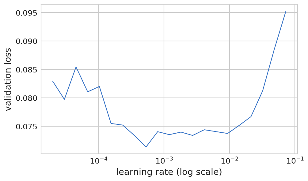
1 2 lrf=learn.lr_find(1e-5 ,100 )
epoch trn_loss val_loss <lambda>
0 1.33405 13.517095 0.5108
关于use_clr的用法:第一个参数是关于精度的,从lr的1/32开始,第二个参数是上升与下降比例。
1 learn.fit(lr, 1 , cycle_len=3 , use_clr=(32 ,5 ))
epoch trn_loss val_loss <lambda>
0 0.322894 0.165013 0.9484
1 0.173385 0.079073 0.9731
2 0.116328 0.074583 0.9748
[array([0.07458]), 0.9747999939918518]
1 lrs = np.array([lr/100 , lr/10 , lr])
1 2 learn.lr_find(lrs/1000 ) learn.sched.plot(0 )
84%|████████▍ | 27/32 [00:05<00:00, 7.20it/s, loss=0.243]
1 learn.fit(lrs/10 , 1 , cycle_len=5 , use_clr=(32 ,5 ))
epoch trn_loss val_loss <lambda>
0 0.075259 0.078922 0.9734
1 0.054866 0.080068 0.9744
2 0.03906 0.079555 0.9764
3 0.028415 0.073445 0.9767
4 0.02 0.075055 0.9771
[array([0.07505]), 0.9770999913215637]
1 2 3 learn.save('mclas' ) learn.load('mclas' )
1 2 3 y = learn.predict() x,_ = next (iter (md.val_dl)) x = to_np(x)
1 2 3 4 5 6 7 8 9 fig, axes = plt.subplots(3 , 4 , figsize=(12 , 8 )) for i,ax in enumerate (axes.flat): ima=md.val_ds.denorm(x)[i] ya = np.nonzero(y[i]>0.4 )[0 ] b = '\n' .join(md.classes[o] for o in ya) ax = show_img(ima, ax=ax) draw_text(ax, (0 ,0 ), b) plt.tight_layout()
Clipping input data to the valid range for imshow with RGB data ([0..1] for floats or [0..255] for integers).
多分类还是比较简单直白的。
目标检测 按照Howard教授讲的,实现一个粗糙版本的SSD,继而进行改进。
训练网络的三要素:
数据
网络结构
Loss函数
1 2 3 4 f_model=resnet34 sz=224 bs=64
数据 构建多分类数据集 1 2 3 4 5 6 multiClass = [[catgoris[p[1 ]] for p in trinAnnos[o]] for o in trinIDs] Id2Catgris = list (catgoris.values()) Catgris2Id = {v:k for k,v in enumerate (Id2Catgris)}
1 2 multiClasses = np.array([np.array([Catgris2Id[p] for p in o]) for o in multiClass])
array([array([6]), array([14, 12]), array([ 1, 1, 14, 14, 14]), ..., array([17, 8, 14, 14, 14]),
array([6]), array([11])], dtype=object)
1 2 3 val_idxs = get_cv_idxs(len (trinFnams)) ((val_mcs,trn_mcs),) = split_by_idx(val_idxs, multiClasses)
构建BBox的数据集 1 MBB_CSV = PATH/'tmp/mbb.csv'
1 2 3 4 5 6 multiBBox = [np.concatenate([p[0 ] for p in trinAnnos[o]]) for o in trinIDs] multiBBoxes = [' ' .join(str (p) for p in o) for o in multiBBox] df = pd.DataFrame({'fn' :[trinFnams[o] for o in trinIDs], 'bbox' :multiBBoxes}, columns=['fn' ,'bbox' ]) df.to_csv(MBB_CSV, index=False )
fn
bbox
0
000012.jpg
96 155 269 350
1
000017.jpg
61 184 198 278 77 89 335 402
2
000023.jpg
229 8 499 244 219 229 499 333 0 1 368 116 1 2 …
3
000026.jpg
124 89 211 336
4
000032.jpg
77 103 182 374 87 132 122 196 179 194 228 212 …
1 2 3 4 5 6 aug_tfms = [RandomRotate(3 , p=0.5 , tfm_y=TfmType.COORD), RandomLighting(0.05 , 0.05 , tfm_y=TfmType.COORD), RandomFlip(tfm_y=TfmType.COORD)] tfms = tfms_from_model(f_model, sz, crop_type=CropType.NO, tfm_y=TfmType.COORD, aug_tfms=aug_tfms) md = ImageClassifierData.from_csv(PATH, JPEGS, MBB_CSV, tfms=tfms, bs=bs, continuous=True , num_workers=4 )
对多分类数据集和BBox数据集进行拼接 1 2 3 4 5 6 7 8 9 10 11 class ConcatLblDataset (Dataset ): def __init__ (self, ds, y2 ): self.ds,self.y2 = ds,y2 self.sz = ds.sz def __len__ (self ): return len (self.ds) def __getitem__ (self, i ): x,y = self.ds[i] return (x, (y,self.y2[i]))
1 2 3 4 5 trn_ds2 = ConcatLblDataset(md.trn_ds, trn_mcs) val_ds2 = ConcatLblDataset(md.val_ds, val_mcs) md.trn_dl.dataset = trn_ds2 md.val_dl.dataset = val_ds2
查看新构建的数据集 1 2 3 4 5 6 7 8 9 10 11 import matplotlib.cm as cmximport matplotlib.colors as mcolorsfrom cycler import cyclerdef get_cmap (N ): color_norm = mcolors.Normalize(vmin=0 , vmax=N-1 ) return cmx.ScalarMappable(norm=color_norm, cmap='Set3' ).to_rgba num_colr = 12 cmap = get_cmap(num_colr) colr_list = [cmap(float (x)) for x in range (num_colr)]
1 2 3 4 5 6 7 8 9 10 11 12 13 def show_ground_truth (ax, im, bbox, clas=None , prs=None , thresh=0.3 ): bb = [bb_hw(o) for o in bbox.reshape(-1 ,4 )] if prs is None : prs = [None ]*len (bb) if clas is None : clas = [None ]*len (bb) ax = show_img(im, ax=ax) for i,(b,c,pr) in enumerate (zip (bb, clas, prs)): if ((b[2 ]>1 ) and (pr is None or pr > thresh)): draw_rect(ax, b, color=colr_list[i%num_colr]) txt = f'{i} : ' if c is not None : txt += ('bg' if c==len (Id2Catgris) else Id2Catgris[c]) if pr is not None : txt += f' {pr:.2 f} ' draw_text(ax, b[:2 ], txt, color=colr_list[i%num_colr])
1 2 3 x,y = to_np(next (iter (md.val_dl))) x = md.val_ds.ds.denorm(x)
1 2 3 4 5 fig, axes = plt.subplots(3 ,4 , figsize=(16 ,12 )) for i,ax in enumerate (axes.flat): show_ground_truth(ax, x[i], y[0 ][i], y[1 ][i]) plt.tight_layout()
Clipping input data to the valid range for imshow with RGB data ([0..1] for floats or [0..255] for integers).
网络结构 先构建简单的模型,后继续改进。先用4x4 anchor。
这里用的是SSD的方式:
SSD的方式是在原有ResNet主干后增加一个stride为2的卷积层,得到4x4的tensor,对每个Tensor做(4+C)的目标检测,共44 (4+C);
YOLO的方式是直接构建16*(4+C)的Linear层。
anchor设置 参数介绍:
anc_grid = how big of a square grid to make (subdivision)
anc_offset = center offsets
anc_x = x coordinates for centers
anc_y = y coordinates for centers
anc_ctrs - the actual coordinates for the grid centers
anc_sizes - size of the quadrants
1 2 3 4 5 6 7 8 9 10 11 12 anc_grid = 4 k = 1 anc_offset = 1 /(anc_grid*2 ) anc_x = np.repeat(np.linspace(anc_offset, 1 - anc_offset, anc_grid), anc_grid) anc_y = np.tile(np.linspace(anc_offset,1 -anc_offset,anc_grid),anc_grid) anc_ctrs = np.tile(np.stack([anc_x,anc_y], axis=1 ), (k,1 )) anc_sizes = np.array([[1 /anc_grid,1 /anc_grid] for i in range (anc_grid*anc_grid)]) anchors = V(np.concatenate([anc_ctrs, anc_sizes], axis=1 ), requires_grad=False ).float ()
1 grid_sizes = V(np.array([1 /anc_grid]), requires_grad=False ).unsqueeze(1 )
1 2 3 4 5 plt.grid(False ) plt.scatter(anc_x, anc_y) plt.xlim(0 , 1 ) plt.ylim(0 , 1 );
Variable containing:
0.1250 0.1250 0.2500 0.2500
0.1250 0.3750 0.2500 0.2500
0.1250 0.6250 0.2500 0.2500
0.1250 0.8750 0.2500 0.2500
0.3750 0.1250 0.2500 0.2500
0.3750 0.3750 0.2500 0.2500
0.3750 0.6250 0.2500 0.2500
0.3750 0.8750 0.2500 0.2500
0.6250 0.1250 0.2500 0.2500
0.6250 0.3750 0.2500 0.2500
0.6250 0.6250 0.2500 0.2500
0.6250 0.8750 0.2500 0.2500
0.8750 0.1250 0.2500 0.2500
0.8750 0.3750 0.2500 0.2500
0.8750 0.6250 0.2500 0.2500
0.8750 0.8750 0.2500 0.2500
[torch.cuda.FloatTensor of size 16x4 (GPU 1)]
1 2 3 def hw2corners (ctr, hw ): return torch.cat([ctr-hw/2 ,ctr+hw/2 ],dim=1 )
1 2 3 anchor_cnr = hw2corners(anchors[:,:2 ],anchors[:,2 :]) anchor_cnr
Variable containing:
0.0000 0.0000 0.2500 0.2500
0.0000 0.2500 0.2500 0.5000
0.0000 0.5000 0.2500 0.7500
0.0000 0.7500 0.2500 1.0000
0.2500 0.0000 0.5000 0.2500
0.2500 0.2500 0.5000 0.5000
0.2500 0.5000 0.5000 0.7500
0.2500 0.7500 0.5000 1.0000
0.5000 0.0000 0.7500 0.2500
0.5000 0.2500 0.7500 0.5000
0.5000 0.5000 0.7500 0.7500
0.5000 0.7500 0.7500 1.0000
0.7500 0.0000 1.0000 0.2500
0.7500 0.2500 1.0000 0.5000
0.7500 0.5000 1.0000 0.7500
0.7500 0.7500 1.0000 1.0000
[torch.cuda.FloatTensor of size 16x4 (GPU 1)]
自定义高级网络层 以ResNet34为主干,追加更多的卷积层。现在是一层卷积层,用于4x4grid。
1 2 n_clas = len (Id2Catgris)+1 n_act = k*(4 +n_clas)
关于flatten的方式 (pytorch中contiguous())[https://blog.csdn.net/appleml/article/details/80143212]:
view只能用在contiguous的variable上。如果在view之前用了transpose, permute等,需要用contiguous()来返回一个contiguous copy。
1 2 3 4 5 6 7 8 9 10 11 12 13 14 15 class StdConv (nn.Module): def __init__ (self, nin, nout, stride=2 , drop=0.1 ): super ().__init__() self.conv = nn.Conv2d(nin, nout, 3 , stride=stride, padding=1 ) self.bn = nn.BatchNorm2d(nout) self.drop = nn.Dropout(drop) def forward (self, x ): return self.drop(self.bn(F.relu(self.conv(x)))) def flatten_conv (x,k ): bs,nf,gx,gy = x.size() x = x.permute(0 ,2 ,3 ,1 ).contiguous() return x.view(bs,-1 ,nf//k)
1 2 3 4 5 6 7 8 9 10 11 12 13 14 class OutConv (nn.Module): def __init__ (self, k, nin, bias ): super ().__init__() self.k = k self.oconv1 = nn.Conv2d(nin, (len (Id2Catgris)+1 )*k, 3 , padding=1 ) self.oconv2 = nn.Conv2d(nin, 4 *k, 3 , padding=1 ) self.oconv1.bias.data.zero_().add_(bias) def forward (self, x ): return [flatten_conv(self.oconv1(x), self.k), flatten_conv(self.oconv2(x), self.k)]
1 2 3 4 5 6 7 8 9 10 11 12 13 14 15 16 class SSD_Head (nn.Module): def __init__ (self, k, bias ): super ().__init__() self.drop = nn.Dropout(0.25 ) self.sconv0 = StdConv(512 ,256 , stride=1 ) self.sconv2 = StdConv(256 ,256 ) self.out = OutConv(k, 256 , bias) def forward (self, x ): x = self.drop(F.relu(x)) x = self.sconv0(x) x = self.sconv2(x) return self.out(x)
1 2 3 4 5 head_reg4 = SSD_Head(k, -3. ) models = ConvnetBuilder(f_model, 0 , 0 , 0 , custom_head=head_reg4) learn = ConvLearner(md, models) learn.opt_fn = optim.Adam
损失函数 损失函数需要先对图像中的目标对应到最后卷积层的其中一个grid中,就可以说是“这个grid是对这一个目标对标的”;
然后进一步地,去衡量坐标的接近程度和分类概率的接近程度。
损失函数:SSD_Loss的计算步骤:
去除zeroPadding
将预测得到的activations转换至BBox(anchor 空间)
计算IOU
将Ground Truth的BBox映射到Anchor 空间
检查是否存在覆盖区域大于0.4的(Ground Truth BBox与4x4的anchors)
寻找匹配的anchor和分类下标
对于为匹配到的,定位background类别
L1损失用于定位,二分交叉熵用于分类
多分类损失函数 1 2 3 4 5 6 7 8 9 10 11 12 13 14 15 16 17 18 def one_hot_embedding (labels, num_classes ): return torch.eye(num_classes)[labels.data.cpu()] class BCE_Loss (nn.Module): def __init__ (self, num_classes ): super ().__init__() self.num_classes = num_classes def forward (self, pred, targ ): t = one_hot_embedding(targ, self.num_classes+1 ) t = V(t[:,:-1 ].contiguous()) x = pred[:,:-1 ] w = self.get_weight(x,t) return F.binary_cross_entropy_with_logits(x, t, w, size_average=False )/self.num_classes def get_weight (self,x,t ): return None
1 2 loss_f = BCE_Loss(len (Id2Catgris))
IOU 计算(定位损失函数) 1 2 3 4 5 6 7 8 9 10 11 12 13 14 15 def intersect (box_a, box_b ): max_xy = torch.min (box_a[:, None , 2 :], box_b[None , :, 2 :]) min_xy = torch.max (box_a[:, None , :2 ], box_b[None , :, :2 ]) inter = torch.clamp((max_xy - min_xy), min =0 ) return inter[:, :, 0 ] * inter[:, :, 1 ] def box_sz (b ): return ((b[:, 2 ]-b[:, 0 ]) * (b[:, 3 ]-b[:, 1 ]))def jaccard (box_a, box_b ): inter = intersect(box_a, box_b) union = box_sz(box_a).unsqueeze(1 ) + box_sz(box_b).unsqueeze(0 ) - inter return inter / union
1 2 3 4 5 6 7 8 9 10 11 12 13 14 15 16 17 18 19 20 21 22 23 24 25 26 27 28 29 30 31 32 33 34 35 36 37 38 39 40 41 42 43 44 45 46 47 48 49 50 51 52 53 54 55 56 57 58 59 60 61 62 63 64 65 66 67 68 69 70 71 72 def get_y (bbox,clas ): bbox = bbox.view(-1 ,4 )/sz bb_keep = ((bbox[:,2 ]-bbox[:,0 ])>0 ).nonzero()[:,0 ] return bbox[bb_keep],clas[bb_keep] def actn_to_bb (actn, anchors ): actn_bbs = torch.tanh(actn) actn_centers = (actn_bbs[:,:2 ]/2 * grid_sizes) + anchors[:,:2 ] actn_hw = (actn_bbs[:,2 :]/2 +1 ) * anchors[:,2 :] return hw2corners(actn_centers, actn_hw) def map_to_ground_truth (overlaps, print_it=False ): prior_overlap, prior_idx = overlaps.max (1 ) if print_it: print (prior_overlap) gt_overlap, gt_idx = overlaps.max (0 ) gt_overlap[prior_idx] = 1.99 for i,o in enumerate (prior_idx): gt_idx[o] = i return gt_overlap,gt_idx def ssd_1_loss (b_c,b_bb,bbox,clas,print_it=False ): bbox,clas = get_y(bbox,clas) a_ic = actn_to_bb(b_bb, anchors) overlaps = jaccard(bbox.data, anchor_cnr.data) gt_overlap,gt_idx = map_to_ground_truth(overlaps,print_it) gt_clas = clas[gt_idx] pos = gt_overlap > 0.4 pos_idx = torch.nonzero(pos)[:,0 ] gt_clas[1 -pos] = len (Id2Catgris) gt_bbox = bbox[gt_idx] loc_loss = ((a_ic[pos_idx] - gt_bbox[pos_idx]).abs ()).mean() clas_loss = loss_f(b_c, gt_clas) return loc_loss, clas_loss
1
2
3
4
5
6
7
8
9
10
11
12
13
def ssd_loss (pred,targ,print_it=False ): lcs,lls = 0. ,0. for b_c,b_bb,bbox,clas in zip (*pred,*targ): loc_loss,clas_loss = ssd_1_loss(b_c,b_bb,bbox,clas,print_it) lls += loc_loss lcs += clas_loss if print_it: print (f'loc: {lls.data[0 ]} , clas: {lcs.data[0 ]} ' ) return lls+lcs
Loss测试 确保loss函数可行
1 2 x,y = next (iter (md.val_dl)) x,y = V(x),V(y)
1 2 for i,o in enumerate (y): y[i] = o.cuda()learn.model.cuda()
Sequential(
(0): Conv2d(3, 64, kernel_size=(7, 7), stride=(2, 2), padding=(3, 3), bias=False)
(1): BatchNorm2d(64, eps=1e-05, momentum=0.1, affine=True)
(2): ReLU(inplace)
(3): MaxPool2d(kernel_size=(3, 3), stride=(2, 2), padding=(1, 1), dilation=(1, 1), ceil_mode=False)
(4): Sequential(
(0): BasicBlock(
(conv1): Conv2d(64, 64, kernel_size=(3, 3), stride=(1, 1), padding=(1, 1), bias=False)
(bn1): BatchNorm2d(64, eps=1e-05, momentum=0.1, affine=True)
(relu): ReLU(inplace)
(conv2): Conv2d(64, 64, kernel_size=(3, 3), stride=(1, 1), padding=(1, 1), bias=False)
(bn2): BatchNorm2d(64, eps=1e-05, momentum=0.1, affine=True)
)
(1): BasicBlock(
(conv1): Conv2d(64, 64, kernel_size=(3, 3), stride=(1, 1), padding=(1, 1), bias=False)
(bn1): BatchNorm2d(64, eps=1e-05, momentum=0.1, affine=True)
(relu): ReLU(inplace)
(conv2): Conv2d(64, 64, kernel_size=(3, 3), stride=(1, 1), padding=(1, 1), bias=False)
(bn2): BatchNorm2d(64, eps=1e-05, momentum=0.1, affine=True)
)
(2): BasicBlock(
(conv1): Conv2d(64, 64, kernel_size=(3, 3), stride=(1, 1), padding=(1, 1), bias=False)
(bn1): BatchNorm2d(64, eps=1e-05, momentum=0.1, affine=True)
(relu): ReLU(inplace)
(conv2): Conv2d(64, 64, kernel_size=(3, 3), stride=(1, 1), padding=(1, 1), bias=False)
(bn2): BatchNorm2d(64, eps=1e-05, momentum=0.1, affine=True)
)
)
(5): Sequential(
(0): BasicBlock(
(conv1): Conv2d(64, 128, kernel_size=(3, 3), stride=(2, 2), padding=(1, 1), bias=False)
(bn1): BatchNorm2d(128, eps=1e-05, momentum=0.1, affine=True)
(relu): ReLU(inplace)
(conv2): Conv2d(128, 128, kernel_size=(3, 3), stride=(1, 1), padding=(1, 1), bias=False)
(bn2): BatchNorm2d(128, eps=1e-05, momentum=0.1, affine=True)
(downsample): Sequential(
(0): Conv2d(64, 128, kernel_size=(1, 1), stride=(2, 2), bias=False)
(1): BatchNorm2d(128, eps=1e-05, momentum=0.1, affine=True)
)
)
(1): BasicBlock(
(conv1): Conv2d(128, 128, kernel_size=(3, 3), stride=(1, 1), padding=(1, 1), bias=False)
(bn1): BatchNorm2d(128, eps=1e-05, momentum=0.1, affine=True)
(relu): ReLU(inplace)
(conv2): Conv2d(128, 128, kernel_size=(3, 3), stride=(1, 1), padding=(1, 1), bias=False)
(bn2): BatchNorm2d(128, eps=1e-05, momentum=0.1, affine=True)
)
(2): BasicBlock(
(conv1): Conv2d(128, 128, kernel_size=(3, 3), stride=(1, 1), padding=(1, 1), bias=False)
(bn1): BatchNorm2d(128, eps=1e-05, momentum=0.1, affine=True)
(relu): ReLU(inplace)
(conv2): Conv2d(128, 128, kernel_size=(3, 3), stride=(1, 1), padding=(1, 1), bias=False)
(bn2): BatchNorm2d(128, eps=1e-05, momentum=0.1, affine=True)
)
(3): BasicBlock(
(conv1): Conv2d(128, 128, kernel_size=(3, 3), stride=(1, 1), padding=(1, 1), bias=False)
(bn1): BatchNorm2d(128, eps=1e-05, momentum=0.1, affine=True)
(relu): ReLU(inplace)
(conv2): Conv2d(128, 128, kernel_size=(3, 3), stride=(1, 1), padding=(1, 1), bias=False)
(bn2): BatchNorm2d(128, eps=1e-05, momentum=0.1, affine=True)
)
)
(6): Sequential(
(0): BasicBlock(
(conv1): Conv2d(128, 256, kernel_size=(3, 3), stride=(2, 2), padding=(1, 1), bias=False)
(bn1): BatchNorm2d(256, eps=1e-05, momentum=0.1, affine=True)
(relu): ReLU(inplace)
(conv2): Conv2d(256, 256, kernel_size=(3, 3), stride=(1, 1), padding=(1, 1), bias=False)
(bn2): BatchNorm2d(256, eps=1e-05, momentum=0.1, affine=True)
(downsample): Sequential(
(0): Conv2d(128, 256, kernel_size=(1, 1), stride=(2, 2), bias=False)
(1): BatchNorm2d(256, eps=1e-05, momentum=0.1, affine=True)
)
)
(1): BasicBlock(
(conv1): Conv2d(256, 256, kernel_size=(3, 3), stride=(1, 1), padding=(1, 1), bias=False)
(bn1): BatchNorm2d(256, eps=1e-05, momentum=0.1, affine=True)
(relu): ReLU(inplace)
(conv2): Conv2d(256, 256, kernel_size=(3, 3), stride=(1, 1), padding=(1, 1), bias=False)
(bn2): BatchNorm2d(256, eps=1e-05, momentum=0.1, affine=True)
)
(2): BasicBlock(
(conv1): Conv2d(256, 256, kernel_size=(3, 3), stride=(1, 1), padding=(1, 1), bias=False)
(bn1): BatchNorm2d(256, eps=1e-05, momentum=0.1, affine=True)
(relu): ReLU(inplace)
(conv2): Conv2d(256, 256, kernel_size=(3, 3), stride=(1, 1), padding=(1, 1), bias=False)
(bn2): BatchNorm2d(256, eps=1e-05, momentum=0.1, affine=True)
)
(3): BasicBlock(
(conv1): Conv2d(256, 256, kernel_size=(3, 3), stride=(1, 1), padding=(1, 1), bias=False)
(bn1): BatchNorm2d(256, eps=1e-05, momentum=0.1, affine=True)
(relu): ReLU(inplace)
(conv2): Conv2d(256, 256, kernel_size=(3, 3), stride=(1, 1), padding=(1, 1), bias=False)
(bn2): BatchNorm2d(256, eps=1e-05, momentum=0.1, affine=True)
)
(4): BasicBlock(
(conv1): Conv2d(256, 256, kernel_size=(3, 3), stride=(1, 1), padding=(1, 1), bias=False)
(bn1): BatchNorm2d(256, eps=1e-05, momentum=0.1, affine=True)
(relu): ReLU(inplace)
(conv2): Conv2d(256, 256, kernel_size=(3, 3), stride=(1, 1), padding=(1, 1), bias=False)
(bn2): BatchNorm2d(256, eps=1e-05, momentum=0.1, affine=True)
)
(5): BasicBlock(
(conv1): Conv2d(256, 256, kernel_size=(3, 3), stride=(1, 1), padding=(1, 1), bias=False)
(bn1): BatchNorm2d(256, eps=1e-05, momentum=0.1, affine=True)
(relu): ReLU(inplace)
(conv2): Conv2d(256, 256, kernel_size=(3, 3), stride=(1, 1), padding=(1, 1), bias=False)
(bn2): BatchNorm2d(256, eps=1e-05, momentum=0.1, affine=True)
)
)
(7): Sequential(
(0): BasicBlock(
(conv1): Conv2d(256, 512, kernel_size=(3, 3), stride=(2, 2), padding=(1, 1), bias=False)
(bn1): BatchNorm2d(512, eps=1e-05, momentum=0.1, affine=True)
(relu): ReLU(inplace)
(conv2): Conv2d(512, 512, kernel_size=(3, 3), stride=(1, 1), padding=(1, 1), bias=False)
(bn2): BatchNorm2d(512, eps=1e-05, momentum=0.1, affine=True)
(downsample): Sequential(
(0): Conv2d(256, 512, kernel_size=(1, 1), stride=(2, 2), bias=False)
(1): BatchNorm2d(512, eps=1e-05, momentum=0.1, affine=True)
)
)
(1): BasicBlock(
(conv1): Conv2d(512, 512, kernel_size=(3, 3), stride=(1, 1), padding=(1, 1), bias=False)
(bn1): BatchNorm2d(512, eps=1e-05, momentum=0.1, affine=True)
(relu): ReLU(inplace)
(conv2): Conv2d(512, 512, kernel_size=(3, 3), stride=(1, 1), padding=(1, 1), bias=False)
(bn2): BatchNorm2d(512, eps=1e-05, momentum=0.1, affine=True)
)
(2): BasicBlock(
(conv1): Conv2d(512, 512, kernel_size=(3, 3), stride=(1, 1), padding=(1, 1), bias=False)
(bn1): BatchNorm2d(512, eps=1e-05, momentum=0.1, affine=True)
(relu): ReLU(inplace)
(conv2): Conv2d(512, 512, kernel_size=(3, 3), stride=(1, 1), padding=(1, 1), bias=False)
(bn2): BatchNorm2d(512, eps=1e-05, momentum=0.1, affine=True)
)
)
(8): SSD_Head(
(drop): Dropout(p=0.25)
(sconv0): StdConv(
(conv): Conv2d(512, 256, kernel_size=(3, 3), stride=(1, 1), padding=(1, 1))
(bn): BatchNorm2d(256, eps=1e-05, momentum=0.1, affine=True)
(drop): Dropout(p=0.1)
)
(sconv2): StdConv(
(conv): Conv2d(256, 256, kernel_size=(3, 3), stride=(2, 2), padding=(1, 1))
(bn): BatchNorm2d(256, eps=1e-05, momentum=0.1, affine=True)
(drop): Dropout(p=0.1)
)
(out): OutConv(
(oconv1): Conv2d(256, 21, kernel_size=(3, 3), stride=(1, 1), padding=(1, 1))
(oconv2): Conv2d(256, 4, kernel_size=(3, 3), stride=(1, 1), padding=(1, 1))
)
)
)
1 ssd_loss(batch, y, True )
0.1947
0.1168
0.2652
[torch.cuda.FloatTensor of size 3 (GPU 1)]
0.2885
0.0888
[torch.cuda.FloatTensor of size 2 (GPU 1)]
...
略
...
1.00000e-02 *
6.3919
9.1493
[torch.cuda.FloatTensor of size 2 (GPU 1)]
0.4062
0.2180
0.1307
0.5762
0.1524
0.4794
[torch.cuda.FloatTensor of size 6 (GPU 1)]
0.1128
[torch.cuda.FloatTensor of size 1 (GPU 1)]
loc: 10.124164581298828, clas: 74.17005157470703
Variable containing:
84.2942
[torch.cuda.FloatTensor of size 1 (GPU 1)]
训练模型 1 2 3 learn.crit = ssd_loss lr = 3e-3 lrs = np.array([lr/100 ,lr/10 ,lr])
1 2 learn.lr_find(lrs/1000 ,1. ) learn.sched.plot(1 )
epoch trn_loss val_loss
0 165.921224 30391.076109
1 learn.fit(lr, 1 , cycle_len=5 , use_clr=(20 ,10 ))
epoch trn_loss val_loss
0 43.098326 34.007883
1 33.96893 28.336332
2 29.650869 26.937769
3 26.758102 26.563267
4 24.590307 26.008181
[array([26.00818])]
1 2 3 learn.save('0' ) learn.load('0' )
测试模型 直接预测 1 2 3 4 5 x,y = next (iter (md.val_dl)) x,y = V(x),V(y) learn.model.eval () batch = learn.model(x) b_clas,b_bb = batch
1 b_clas.size(),b_bb.size()
(torch.Size([64, 16, 21]), torch.Size([64, 16, 4]))
1 2 3 4 5 6 7 idx=7 b_clasi = b_clas[idx] b_bboxi = b_bb[idx] ima=md.val_ds.ds.denorm(to_np(x))[idx] bbox,clas = get_y(y[0 ][idx], y[1 ][idx]) bbox,clas
(Variable containing:
0.6786 0.4866 0.9911 0.6250
0.7098 0.0848 0.9911 0.5491
0.5134 0.8304 0.6696 0.9063
[torch.cuda.FloatTensor of size 3x4 (GPU 1)], Variable containing:
8
10
17
[torch.cuda.LongTensor of size 3 (GPU 1)])
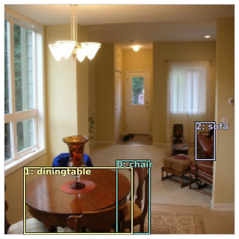
1 2 3 4 def torch_gt (ax, ima, bbox, clas, prs=None , thresh=0.4 ): return show_ground_truth(ax, ima, to_np((bbox*224 ).long()), to_np(clas), to_np(prs) if prs is not None else None , thresh)
1 2 3 fig, ax = plt.subplots(figsize=(7 ,7 )) torch_gt(ax, ima, bbox, clas)
1 2 3 fig, ax = plt.subplots(figsize=(7 ,7 )) torch_gt(ax, ima, anchor_cnr, b_clasi.max (1 )[1 ])
过一遍流程,加强理解 Variable containing:
0.2500
[torch.cuda.FloatTensor of size 1x1 (GPU 1)]
Variable containing:
0.1250 0.1250 0.2500 0.2500
0.1250 0.3750 0.2500 0.2500
0.1250 0.6250 0.2500 0.2500
0.1250 0.8750 0.2500 0.2500
0.3750 0.1250 0.2500 0.2500
0.3750 0.3750 0.2500 0.2500
0.3750 0.6250 0.2500 0.2500
0.3750 0.8750 0.2500 0.2500
0.6250 0.1250 0.2500 0.2500
0.6250 0.3750 0.2500 0.2500
0.6250 0.6250 0.2500 0.2500
0.6250 0.8750 0.2500 0.2500
0.8750 0.1250 0.2500 0.2500
0.8750 0.3750 0.2500 0.2500
0.8750 0.6250 0.2500 0.2500
0.8750 0.8750 0.2500 0.2500
[torch.cuda.FloatTensor of size 16x4 (GPU 1)]
1 2 a_ic = actn_to_bb(b_bboxi, anchors)
1 2 3 fig, ax = plt.subplots(figsize=(7 ,7 )) torch_gt(ax, ima, a_ic, b_clasi.max (1 )[1 ], b_clasi.max (1 )[0 ].sigmoid(), thresh=0.0 )
1 2 3 overlaps = jaccard(bbox.data, anchor_cnr.data) overlaps
Columns 0 to 9
0.0000 0.0000 0.0000 0.0000 0.0000 0.0000 0.0000 0.0000 0.0000 0.0091
0.0000 0.0000 0.0000 0.0000 0.0000 0.0000 0.0000 0.0000 0.0356 0.0549
0.0000 0.0000 0.0000 0.0000 0.0000 0.0000 0.0000 0.0000 0.0000 0.0000
Columns 10 to 15
0.0922 0.0000 0.0000 0.0315 0.3985 0.0000
0.0103 0.0000 0.2598 0.4538 0.0653 0.0000
0.0000 0.1897 0.0000 0.0000 0.0000 0.0000
[torch.cuda.FloatTensor of size 3x16 (GPU 1)]
1 2 3 gt_overlap,gt_idx = map_to_ground_truth(overlaps) gt_overlap,gt_idx
(
0.0000
0.0000
0.0000
0.0000
0.0000
0.0000
0.0000
0.0000
0.0356
0.0549
0.0922
1.9900
0.2598
1.9900
1.9900
0.0000
[torch.cuda.FloatTensor of size 16 (GPU 1)],
0
0
0
0
0
0
0
0
1
1
0
2
1
1
0
0
[torch.cuda.LongTensor of size 16 (GPU 1)])
1 2 gt_clas = clas[gt_idx]; gt_clas
Variable containing:
8
8
8
8
8
8
8
8
10
10
8
17
10
10
8
8
[torch.cuda.LongTensor of size 16 (GPU 1)]
1 2 3 4 5 thresh = 0.5 pos = gt_overlap > thresh pos_idx = torch.nonzero(pos)[:,0 ] neg_idx = torch.nonzero(1 -pos)[:,0 ] pos_idx
11
13
14
[torch.cuda.LongTensor of size 3 (GPU 1)]
1 2 3 gt_clas[1 -pos] = len (Id2Catgris) [Id2Catgris[o] if o<len (Id2Catgris) else 'bg' for o in gt_clas.data]
['bg',
'bg',
'bg',
'bg',
'bg',
'bg',
'bg',
'bg',
'bg',
'bg',
'bg',
'sofa',
'bg',
'diningtable',
'chair',
'bg']
1 2 3 4 5 gt_bbox = bbox[gt_idx] loc_loss = ((a_ic[pos_idx] - gt_bbox[pos_idx]).abs ()).mean() clas_loss = F.cross_entropy(b_clasi, gt_clas) loc_loss,clas_loss
(Variable containing:
1.00000e-02 *
6.3615
[torch.cuda.FloatTensor of size 1 (GPU 1)], Variable containing:
0.9142
[torch.cuda.FloatTensor of size 1 (GPU 1)])
1 2 3 4 5 6 7 8 9 10 fig, axes = plt.subplots(3 , 4 , figsize=(16 , 12 )) for idx,ax in enumerate (axes.flat): ima=md.val_ds.ds.denorm(to_np(x))[idx] bbox,clas = get_y(y[0 ][idx], y[1 ][idx]) ima=md.val_ds.ds.denorm(to_np(x))[idx] bbox,clas = get_y(bbox,clas); bbox,clas a_ic = actn_to_bb(b_bb[idx], anchors) torch_gt(ax, ima, a_ic, b_clas[idx].max (1 )[1 ], b_clas[idx].max (1 )[0 ].sigmoid(), 0.01 ) plt.tight_layout()
Clipping input data to the valid range for imshow with RGB data ([0..1] for floats or [0..255] for integers).
进一步的改进:更多的anchor box 提升的途径:
不同大小的Anchor Boxes -> anc_zooms
不同长宽比的Anchor Boxes -> anc_ratios
使用更多的卷积层来产生Anchor Boxes -> anc_grids
创建更多的anchor 1 2 3 4 5 6 7 8 9 10 11 12 13 14 15 16 17 anc_grids = [4 ,2 ,1 ] anc_zooms = [0.7 , 1. , 1.3 ] anc_ratios = [(1. ,1. ), (1. ,0.5 ), (0.5 ,1. )] anchor_scales = [(anz*i, anz*j) for anz in anc_zooms for (i,j) in anc_ratios] k = len (anchor_scales) anc_offsets = [1 /(o*2 ) for o in anc_grids] k
9
1 2 3 4 5 6 anc_x = np.concatenate([np.repeat(np.linspace(ao, 1 -ao,ag),ag) for ao,ag in zip (anc_offsets, anc_grids)]) anc_y = np.concatenate([np.tile(np.linspace(ao,1 -ao,ag), ag) for ao,ag in zip (anc_offsets,anc_grids)]) anc_ctrs = np.repeat(np.stack([anc_x,anc_y],axis=1 ),k,axis=0 )
1 2 3 4 5 6 7 8 9 10 11 12 13 14 15 anc_sizes = np.concatenate([np.array([[o/ag,p/ag] for i in range (ag*ag) for o,p in anchor_scales]) for ag in anc_grids]) grid_sizes = V(np.concatenate([np.array([ 1 /ag for i in range (ag*ag) for o,p in anchor_scales]) for ag in anc_grids]), requires_grad=False ).unsqueeze(1 ) anchors = V(np.concatenate([anc_ctrs, anc_sizes], axis=1 ), requires_grad=False ).float () anchor_cnr = hw2corners(anchors[:,:2 ],anchors[:,2 :])
1 2 x,y=to_np(next (iter (md.val_dl))) x=md.val_ds.ds.denorm(x)
1 a=np.reshape((to_np(anchor_cnr) + to_np(torch.randn(*anchor_cnr.size()))*0.01 )*224 , -1 )
1 2 fig, ax = plt.subplots(figsize=(7 ,7 )) show_ground_truth(ax, x[0 ], a)
创建模型
理一下思路:
已经有了GroundTruth(包括4个BBox坐标点和1个分类的集合);
已经有了一个神经网络可以接收输入图像,并且得到输出activation(激励);
activations与Ground Truth进行对比,计算loss,然后就是求导更新权重;
【匹配问题】定义的损失函数loss function能够比较activation和ground truth,计算得到的值用于衡量activation的好坏。为此,对于ground truth中的每个Object,需要决定一组(4+C)的activation与之对比。
因为使用的SSD的方式,所以匹配的anchorBox并不是随意的,用于匹配的activation,其感受野(reception filed)需要与ground truth中的Object所处的位置具有最大的重叠。
匹配问题解决后,即Loss解决后,其他的操作和单目标检测相同。
关于参数k的使用:
grid cell可以使不同大小的(anc_grid),grid cell中可以有不同长宽比和缩放比的anchor box;
anchor box的数目即对应了卷积层activation的组数目,但并不表示每个卷积层需要那么多组activation,因为4x4的卷积层有16组,2x2的卷积层有4组,1x1的卷积层有1组,这样就有了1+4+16组。
接下来只需要知道参数k,k表示的是长宽比和缩放比的组合数。这样,1xk+4xk+16xk,就是全部的anchor box数目了。
1 2 3 4 5 6 7 8 9 10 11 12 13 14 15 16 17 18 19 20 21 22 23 24 25 26 27 28 29 30 31 32 33 34 35 drop=0.4 class SSD_MultiHead (nn.Module): def __init__ (self, k, bias ): super ().__init__() self.drop = nn.Dropout(drop) self.sconv0 = StdConv(512 ,256 , stride=1 , drop=drop) self.sconv1 = StdConv(256 ,256 , drop=drop) self.sconv2 = StdConv(256 ,256 , drop=drop) self.sconv3 = StdConv(256 ,256 , drop=drop) self.out0 = OutConv(k, 256 , bias) self.out1 = OutConv(k, 256 , bias) self.out2 = OutConv(k, 256 , bias) self.out3 = OutConv(k, 256 , bias) def forward (self, x ): x = self.drop(F.relu(x)) x = self.sconv0(x) x = self.sconv1(x) o1c,o1l = self.out1(x) x = self.sconv2(x) o2c,o2l = self.out2(x) x = self.sconv3(x) o3c,o3l = self.out3(x) return [torch.cat([o1c,o2c,o3c], dim=1 ), torch.cat([o1l,o2l,o3l], dim=1 )] head_reg4 = SSD_MultiHead(k, -4. ) models = ConvnetBuilder(f_model, 0 , 0 , 0 , custom_head=head_reg4) learn = ConvLearner(md, models) learn.opt_fn = optim.Adam
训练和测试 1 2 3 learn.crit = ssd_loss lr = 1e-2 lrs = np.array([lr/100 ,lr/10 ,lr])
1 2 3 x,y = next (iter (md.val_dl)) x,y = V(x),V(y) batch = learn.model(V(x))
1 batch[0 ].size(),batch[1 ].size()
(torch.Size([64, 189, 21]), torch.Size([64, 189, 4]))
1 2 ssd_loss(batch, y, True )
0.5598
0.7922
0.3095
[torch.cuda.FloatTensor of size 3 (GPU 1)]
0.6075
0.7035
[torch.cuda.FloatTensor of size 2 (GPU 1)]
0.7764
[torch.cuda.FloatTensor of size 1 (GPU 1)]
...
略
...
0.9778
0.7173
[torch.cuda.FloatTensor of size 2 (GPU 1)]
0.4372
0.5850
0.2238
0.5762
0.6364
0.4794
[torch.cuda.FloatTensor of size 6 (GPU 1)]
0.7610
[torch.cuda.FloatTensor of size 1 (GPU 1)]
loc: 7.328256130218506, clas: 325.04620361328125
Variable containing:
332.3745
[torch.cuda.FloatTensor of size 1 (GPU 1)]
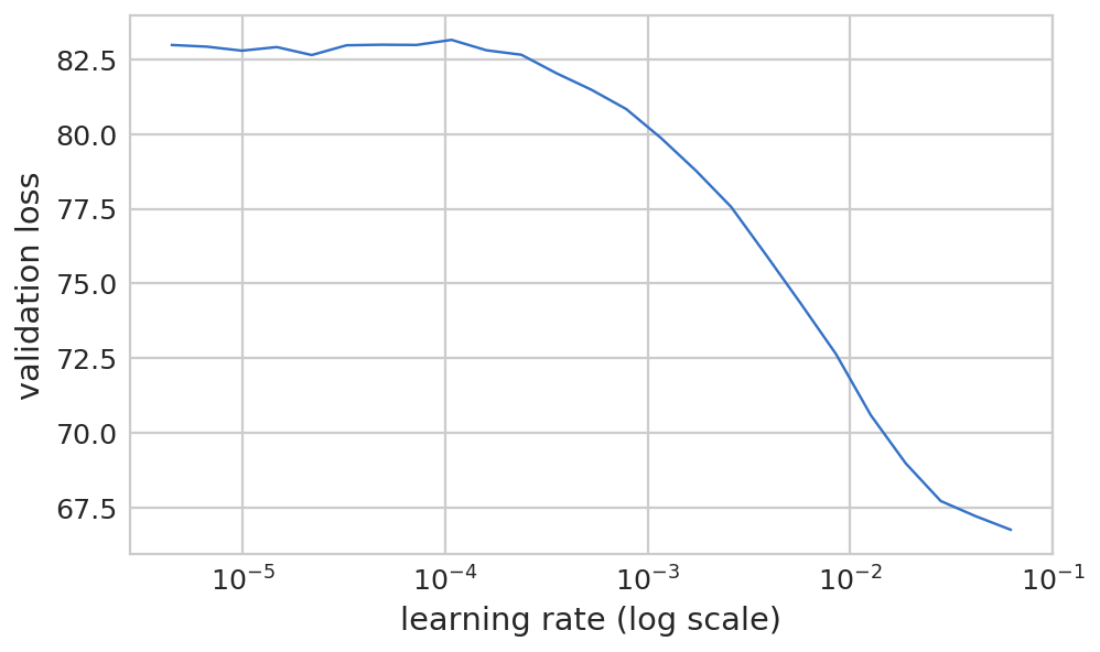
1 2 learn.lr_find(lrs/1000 ,1. ) learn.sched.plot(n_skip_end=2 )
epoch trn_loss val_loss
0 428.072253 7912290.892
1 learn.fit(lrs, 1 , cycle_len=4 , use_clr=(20 ,8 ))
epoch trn_loss val_loss
0 162.041704 142.485135
1 129.785899 104.201066
2 110.773746 93.877435
3 98.444387 89.302771
[array([89.30277])]
1 2 learn.freeze_to(-2 ) learn.fit(lrs/2 , 1 , cycle_len=4 , use_clr=(20 ,8 ))
epoch trn_loss val_loss
0 91.526261 110.951304
1 86.313832 88.162423
2 78.734507 82.294672
3 71.840125 77.196213
[array([77.19621])]
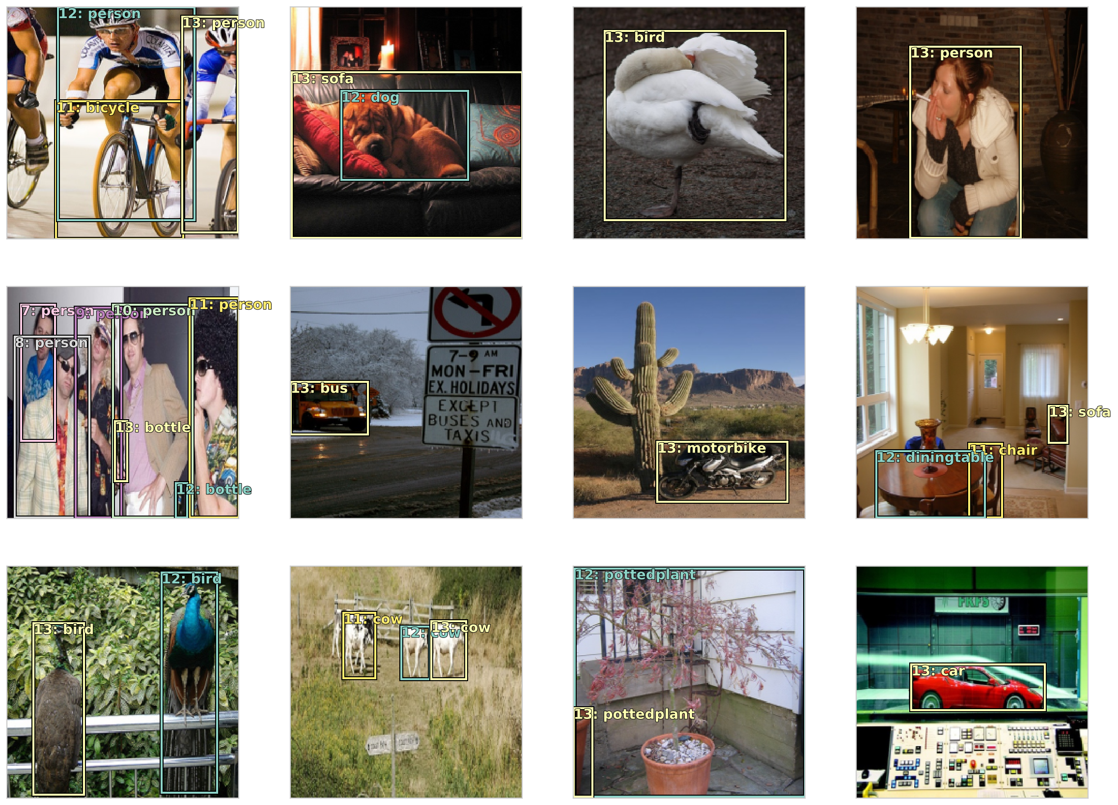
1 2 3 4 5 6 7 8 9 10 11 12 13 14 x,y = next (iter (md.val_dl)) y = V(y) batch = learn.model(V(x)) b_clas,b_bb = batch x = to_np(x) fig, axes = plt.subplots(3 , 4 , figsize=(16 , 12 )) for idx,ax in enumerate (axes.flat): ima=md.val_ds.ds.denorm(x)[idx] bbox,clas = get_y(y[0 ][idx], y[1 ][idx]) a_ic = actn_to_bb(b_bb[idx], anchors) torch_gt(ax, ima, a_ic, b_clas[idx].max (1 )[1 ], b_clas[idx].max (1 )[0 ].sigmoid(), 0.21 ) plt.tight_layout()
Clipping input data to the valid range for imshow with RGB data ([0..1] for floats or [0..255] for integers).
上面打印出来的是置信度大于0.2的,一些图看起来很有改进空间。
Focal Loss 论文《Focal Loss for Dense Object Detection》https://arxiv.org/abs/1708.02002
Focal Loss 就是一个解决分类问题中类别不平衡、分类难度差异的一个 loss。
相关博文:《何恺明大神的「Focal Loss」,如何更好地理解?》
定义Focal Loss 1 2 3 4 5 6 7 8 9 10 class FocalLoss (BCE_Loss ): def get_weight (self,x,t ): alpha,gamma = 0.25 ,1 p = x.sigmoid() pt = p*t + (1 -p)*(1 -t) w = alpha*t + (1 -alpha)*(1 -t) return w * (1 -pt).pow (gamma) loss_f = FocalLoss(len (Id2Catgris))
1 2 3 4 5 x,y = next (iter (md.val_dl)) x,y = V(x),V(y) batch = learn.model(x) ssd_loss(batch, y, True )
0.5598
0.7922
0.3095
[torch.cuda.FloatTensor of size 3 (GPU 1)]
0.6075
0.7035
[torch.cuda.FloatTensor of size 2 (GPU 1)]
0.7764
[torch.cuda.FloatTensor of size 1 (GPU 1)]
...
略
...
0.9778
0.7173
[torch.cuda.FloatTensor of size 2 (GPU 1)]
0.4372
0.5850
0.2238
0.5762
0.6364
0.4794
[torch.cuda.FloatTensor of size 6 (GPU 1)]
0.7610
[torch.cuda.FloatTensor of size 1 (GPU 1)]
loc: 4.548206329345703, clas: 16.757646560668945
Variable containing:
21.3059
[torch.cuda.FloatTensor of size 1 (GPU 1)]
训练和测试 1 2 learn.lr_find(lrs/1000 ,1. ) learn.sched.plot(n_skip_end=1 )
91%|█████████ | 29/32 [00:17<00:01, 1.79it/s, loss=26.2]
1 learn.fit(lrs, 1 , cycle_len=10 , use_clr=(20 ,10 ))
epoch trn_loss val_loss
0 18.807729 34.186557
1 20.281371 21.784252
2 19.392129 19.913282
3 18.172636 18.960041
4 16.900487 18.011309
5 15.716368 17.454738
6 14.717347 16.916381
7 13.727865 16.583986
8 12.809763 16.275561
9 12.093133 16.069795
[array([16.06979])]
1 2 3 learn.save('fl0' ) learn.load('fl0' )
1 2 3 learn.freeze_to(-2 ) learn.fit(lrs/4 , 1 , cycle_len=10 , use_clr=(20 ,10 ))
epoch trn_loss val_loss
0 11.201092 16.542418
1 11.259083 16.820294
2 11.088501 16.641474
3 10.854862 16.461994
4 10.569602 16.541856
5 10.20212 16.264861
6 9.873908 16.241601
7 9.576044 16.212703
8 9.294867 16.157229
9 9.012196 16.187851
[array([16.18785])]
1 2 learn.save('drop4' ) learn.load('drop4' )
1 2 3 4 5 6 7 8 9 10 11 12 13 14 15 16 17 def plot_results (thresh ): x,y = next (iter (md.val_dl)) y = V(y) batch = learn.model(V(x)) b_clas,b_bb = batch x = to_np(x) fig, axes = plt.subplots(3 , 4 , figsize=(16 , 12 )) for idx,ax in enumerate (axes.flat): ima=md.val_ds.ds.denorm(x)[idx] bbox,clas = get_y(y[0 ][idx], y[1 ][idx]) a_ic = actn_to_bb(b_bb[idx], anchors) clas_pr, clas_ids = b_clas[idx].max (1 ) clas_pr = clas_pr.sigmoid() torch_gt(ax, ima, a_ic, clas_ids, clas_pr, clas_pr.max ().data[0 ]*thresh) plt.tight_layout()
Clipping input data to the valid range for imshow with RGB data ([0..1] for floats or [0..255] for integers).
上面的预测已经差不多了,最后一步就是如何筛选出众多选项中最合适的一个作为结果了。也就是非极大抑制。
非极大抑制(NMS) 按照Howard的说法,NMS好理解,但比较繁琐,他也是直接摘的网上的一段代码。
1 2 3 4 5 6 7 8 9 10 11 12 13 14 15 16 17 18 19 20 21 22 23 24 25 26 27 28 29 30 31 32 33 34 35 36 37 38 39 40 41 42 43 44 45 46 47 48 49 50 def nms (boxes, scores, overlap=0.5 , top_k=100 ): keep = scores.new(scores.size(0 )).zero_().long() if boxes.numel() == 0 : return keep x1 = boxes[:, 0 ] y1 = boxes[:, 1 ] x2 = boxes[:, 2 ] y2 = boxes[:, 3 ] area = torch.mul(x2 - x1, y2 - y1) v, idx = scores.sort(0 ) idx = idx[-top_k:] xx1 = boxes.new() yy1 = boxes.new() xx2 = boxes.new() yy2 = boxes.new() w = boxes.new() h = boxes.new() count = 0 while idx.numel() > 0 : i = idx[-1 ] keep[count] = i count += 1 if idx.size(0 ) == 1 : break idx = idx[:-1 ] torch.index_select(x1, 0 , idx, out=xx1) torch.index_select(y1, 0 , idx, out=yy1) torch.index_select(x2, 0 , idx, out=xx2) torch.index_select(y2, 0 , idx, out=yy2) xx1 = torch.clamp(xx1, min =x1[i]) yy1 = torch.clamp(yy1, min =y1[i]) xx2 = torch.clamp(xx2, max =x2[i]) yy2 = torch.clamp(yy2, max =y2[i]) w.resize_as_(xx2) h.resize_as_(yy2) w = xx2 - xx1 h = yy2 - yy1 w = torch.clamp(w, min =0.0 ) h = torch.clamp(h, min =0.0 ) inter = w*h rem_areas = torch.index_select(area, 0 , idx) union = (rem_areas - inter) + area[i] IoU = inter/union idx = idx[IoU.le(overlap)] return keep, count
1 2 3 4 5 6 x,y = next (iter (md.val_dl)) y = V(y) batch = learn.model(V(x)) b_clas,b_bb = batch x = to_np(x)
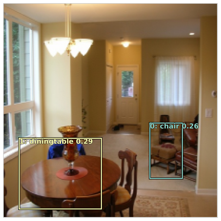
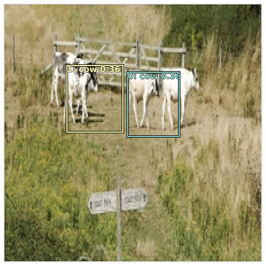
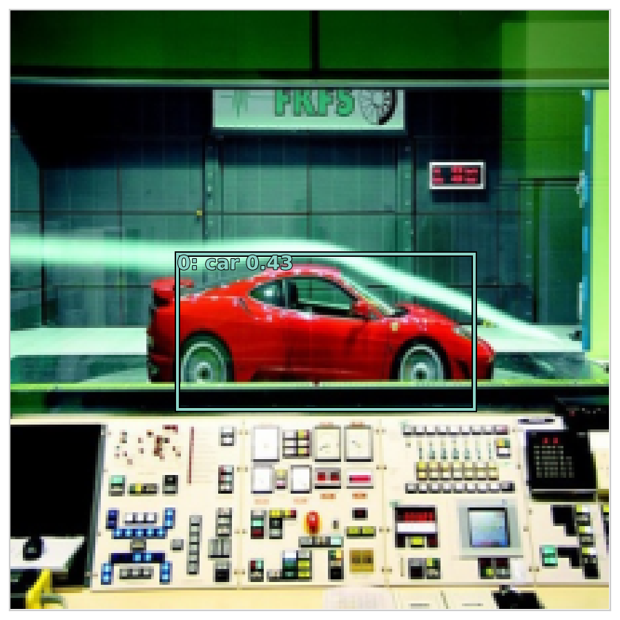
1 2 3 4 5 6 7 8 9 10 11 12 13 14 15 16 17 18 19 20 21 22 23 24 25 26 27 28 29 30 def show_nmf (idx ): ima=md.val_ds.ds.denorm(x)[idx] bbox,clas = get_y(y[0 ][idx], y[1 ][idx]) a_ic = actn_to_bb(b_bb[idx], anchors) clas_pr, clas_ids = b_clas[idx].max (1 ) clas_pr = clas_pr.sigmoid() conf_scores = b_clas[idx].sigmoid().t().data out1,out2,cc = [],[],[] for cl in range (0 , len (conf_scores)-1 ): c_mask = conf_scores[cl] > 0.25 if c_mask.sum () == 0 : continue scores = conf_scores[cl][c_mask] l_mask = c_mask.unsqueeze(1 ).expand_as(a_ic) boxes = a_ic[l_mask].view(-1 , 4 ) ids, count = nms(boxes.data, scores, 0.4 , 50 ) ids = ids[:count] out1.append(scores[ids]) out2.append(boxes.data[ids]) cc.append([cl]*count) if not cc: print (f"{i} : empty array" ) return cc = T(np.concatenate(cc)) out1 = torch.cat(out1) out2 = torch.cat(out2) fig, ax = plt.subplots(figsize=(8 ,8 )) torch_gt(ax, ima, out2, cc, out1, 0.1 )
1 for i in range (12 ): show_nmf(i)
5: empty array
6: empty array
Clipping input data to the valid range for imshow with RGB data ([0..1] for floats or [0..255] for integers).
10: empty array
End 效果还是有待提升,先去看SSD 论文了。
SSD: Single Shot MultiBox Detector