CS131,Homewrok8,Tracking-OpticalFlow

Homework 8

This assignment covers Lukas-Kanade tracking method. Please hand in motion.py and this notebook file to Gradescope.

这份作业是实现Lukas-Kanade光流追踪算法。

# Setup
import numpy as np
from skimage import filters
from skimage.feature import corner_peaks
import matplotlib.pyplot as plt
from matplotlib import rc
from IPython.display import HTML

from __future__ import print_function

%matplotlib inline
#plt.rcParams['figure.figsize'] = (15.0, 12.0) # set default size of plots
plt.rcParams['image.interpolation'] = 'nearest'
plt.rcParams['image.cmap'] = 'gray'

# for auto-reloading extenrnal modules
%load_ext autoreload
%autoreload 2

0. Displaying Video

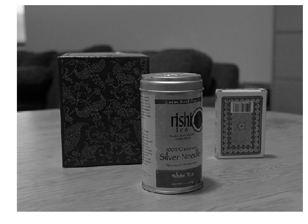
We have done some cool stuff with static images in past assignemnts. Now, let’s turn our attention to videos! For this assignment, the videos are provided as time series of images. We also provide utility functions to load the image frames and visualize them as a short video clip.

Note: You may need to install video codec like FFmpeg. For Linux/Mac, you will be able to install ffmpeg using apt-get or brew. For Windows, you can find the installation instructions here.

用视频来做处理。

此处将图片序列整理成短视频片段。

需要安装ffmpeg。推荐的方式是在anaconda下安装：conda install -c conda-forge ffmpeg

from utils import animated_frames, load_frames
frames = load_frames('images')
ani = animated_frames(frames)
HTML(ani.to_html5_video())

1. Lucas-Kanade Method for Optical Flow

1.1 Deriving optical flow equation

Optical flow methods are used to estimate motion at each pixel location in two consecutive image frames. The optical flow equation at a spatio-temporal point $\mathbf{p}=(x, y, t)$ is given by:

$$ I_x({\mathbf{p}})v_{x} + I_y({\mathbf{p}})v_{y} + I_t({\mathbf{p}}) = 0 $$

,where $I_x$, $I_y$ and $I_t$ are partial derivatives of pixel intensity $I$, and $v_{x}={\Delta x}/{\Delta t}$ and $v_{x}={\Delta x}/{\Delta t}$ are flow vectors.

Let us derive the equation in order to understand what it actually means. First, we make a reasonable assumption (a.k.a. brightness constancy) that the pixel intensity of a moving point stays the same between two consecutive frames with small time difference. Consider pixel intensity $I(x, y, t)$ of a point $(x, y)$ in the first frame $t$. Suppose that the point has moved to $(x+\Delta{x}, y+\Delta{y})$ after $\Delta{t}$. According to the brightness constancy constraint, we can relate intensities of the point in the two frames using the following equation:

$$ I(x,y,t)=I(x+\Delta{x},y+\Delta{y},t+\Delta{t}) $$

• a. Derive the optical flow equation from the brightness constancy equation. Clearly state any assumption you make during derivation.

• b. Can the optical flow equation be solved given two consecutive frames without further assumption? Which values can be computed directly given two consecutive frames? Which values cannot be computed without additional information?

Your answer here: Write your answer in this markdown cell

光流公式的推导

a.

利用灰度不变假设，我们有：

$$ I(x,y,t)=I(x+\Delta{x},y+\Delta{y},t+\Delta{t}) $$

对右边进行泰勒展开，保留一阶项，得：

$$ I(x+\Delta{x},y+\Delta{y},t+\Delta{t}) \approx I(x,y,t) + I_x\Delta{x} + I_y\Delta{y} + I_t\Delta{t} $$

因为我们假设了灰度不变，所以下个时刻的灰度等于之前的灰度，从而：

$$ I_x\Delta{x} + I_y\Delta{y} + I_t\Delta{t} = 0 $$

两边除以$\Delta{t}$ ，得：

$$ I_x \frac{\Delta{x}}{\Delta{t}} + I_y\frac{\Delta{y}}{\Delta{t}} + I_t= 0 $$

其中，$\frac{\Delta{x}}{\Delta{t}}$表示像素在x轴上的运动速度，$\frac{\Delta{y}}{\Delta{t}}$表示像素在y轴上的运动速度，用$v_x$和$v_y$表示，最终得：

$$ I_x({\mathbf{p}})v_{x} + I_y({\mathbf{p}})v_{y} + I_t({\mathbf{p}}) = 0 $$

b.
问：光流方程凭借上式，不做其他假设能够求解？

答：不能求解。

上式中，$I_x$、$I_y$、$I_t$可以经由连续的两幅图像求解，$I_x$表示图像在点P处x方向的梯度，$I_y$表示图像在点P处y方向的梯度，$I_t$表示图像灰度对时间的变化量。

但是仍有两个未知变量$v_x$和$v_y$，最终得到的是一个两个变量的一次方程。

无法求解，需要引入其他约束。

1.2 Overview of Lucas-Kanade method

The Lucas–Kanade method assumes that the motion of the image contents between two frames is approximately constant within a neighborhood of the point $p$ under consideration (spatial coherence).

Consider a neighborhood of $p$, $N(p)={p_1,…,p_n}$ (e.g. 3x3 window around $p$). According to the optical flow equation and spatial coherence assumption, the following should be satisfied:

For every $p_i \in N(p)$,

$$ I_{x}(p_i)v_x + I_{y}(p_i)v_y = -I_{t}(p_i) $$

These equations can be written in matrix form $Av=b$, where

$$ A = \begin{bmatrix} I_{x}(p_1) & I_{y}(p_1)\\ I_{x}(p_2) & I_{y}(p_2)\\ \vdots & \vdots\\ I_{x}(p_n) & I_{y}(p_n) \end{bmatrix} \quad v = \begin{bmatrix} v_{x}\\ v_{y} \end{bmatrix} \quad b = \begin{bmatrix} -I_{t}(p_1)\\ -I_{t}(p_2)\\ \vdots\\ -I_{t}(p_n) \end{bmatrix} $$

Note that this linear system may not have solution for $v$ as it is usually over-determined. Instead, Lucas-Kanade method estimates the flow vector by solving the least-squares problem, $A^{T}Av=A^{T}b$.

• a. What is the condition for this equation to be solvable?
• b. Reason about why Harris corners might be good features to track using Lucas-Kanade method.

Lucas-Kanade算法的思想

上一个光流公式的推导可以得知：求解光流公式需要引入其他约束，而LK光流法的约束就是，假设某一个窗口内的像素具有相同的运动。

如果是采用3x3的窗口，则会另有9个公式，此时采用最小二乘来估计最优的$v_x$和$v_y$即可。

Your answer here: Write your answer in this markdown cell

问题a：方程求解的条件是什么？参见lecture17 PPT

• $A^TA$可逆
• 因为噪声的存在，$A^TA$不能太小
  • $A^TA$的特征值$λ_1$和$λ_2$都不能太小
• $A^TA$应当是well-conditioned
  • $\frac{λ_1}{λ_2} $不能太大，（$λ_1$是较大的特征值）

问题b：为何Harris角点会是LK光流法追踪的好特征？参见lecture17 PPT第25页

因为$M=A^TA$是二阶矩矩阵，$A^TA$的特征向量和特征值与边缘的方向和强度相关。

• 较大的特征值对应的特征向量表示强度变化最快的方向
• 另外一个特征向量则与它正交

1.3 Implementation of Lucas-Kanade method

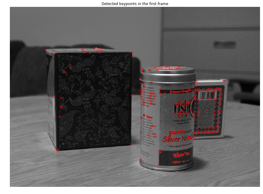
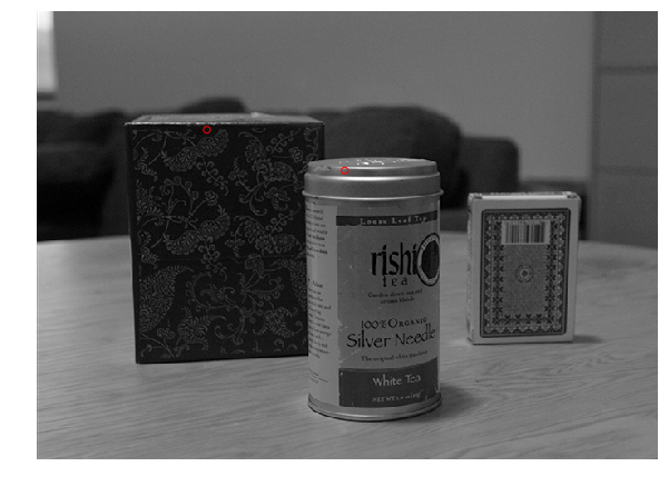
In this section, we are going to implement basic Lucas-Kanade method for feature tracking. In order to do so, we first need to find keypoints to track. Harris corner detector is commonly used to initialize the keypoints to track with Lucas-Kanade method. For this assignment, we are going to use skimage implementation of Harris corner detector.

实现基础版本LK光流

第一步需要找到关键点来进行追踪。

Lucas-Kanade方法通常是使用Harris角点检测器来进行关键点的初始化。

skimage中提供了Harris角点检测的实现。

skimage中的Harris角点检测可以参考：Programming Computer Vision with Python （学习笔记九）

from skimage import filters
from skimage.feature import corner_harris, corner_peaks

frames = load_frames('images')

# Detect keypoints to track

keypoints = corner_peaks(corner_harris(frames[0]),
                         exclude_border=5,
                         threshold_rel=0.01)

# Plot kepoints
plt.figure(figsize=(15,12))
plt.imshow(frames[0])
plt.scatter(keypoints[:,1], keypoints[:,0],
            facecolors='none', edgecolors='r')
plt.axis('off')
plt.title('Detected keypoints in the first frame')
plt.show()

Implement function lucas_kanade in motion.py and run the code cell below. You will be able to see small arrows pointing towards the directions where keypoints are moving.

实现两帧之间的LK光流追踪

from motion import lucas_kanade

# Lucas-Kanade method for optical flow
flow_vectors = lucas_kanade(frames[0], frames[1], keypoints, window_size=5)

# Plot flow vectors
plt.figure(figsize=(15,12))
plt.imshow(frames[0])
plt.axis('off')
plt.title('Optical flow vectors')

# 用箭头标记
for y, x, vy, vx in np.hstack((keypoints, flow_vectors)):
    plt.arrow(x, y, vx, vy, head_width=5, head_length=5, color='b')
    

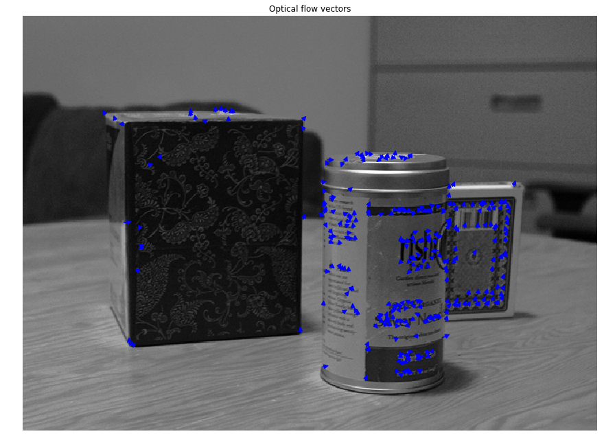
We can estimate the position of the keypoints in the next frame by adding the flow vectors to the keypoints.

通过当前帧关键点的位置和光流的方向，就可以预测下一帧中的关键点的位置

# Plot tracked kepoints
new_keypoints = keypoints + flow_vectors
plt.figure(figsize=(15,12))
plt.imshow(frames[1])
plt.scatter(new_keypoints[:,1], new_keypoints[:,0],
            facecolors='none', edgecolors='r')
plt.axis('off')
plt.title('Tracked keypoints in the second frame')
plt.show()

上图可以看到，光流法预测的第二帧中的特征点地位置还是基本正确的。

1.4 Feature Tracking in multiple frames

Now we can use Lucas-Kanade method to track keypoints across multiple frames. The idea is simple: compute flow vectors at keypoints in $i$-th frame, and add the flow vectors to the points to keep track of the points in $i+1$-th frame. We have provided the function track_features for you. First, run the code cell below. You will notice that some of the points just drift away and are not tracked very well.

Instead of keeping these ‘bad’ tracks, we would want to somehow declare some points are ‘lost’ and just discard them. One simple way to is to compare the patches around tracked points in two subsequent frames. If the patch around a point is NOT similar to the patch around the corresponding point in the next frame, then we declare the point to be lost. Here, we are going to use mean squared error between two normalized patches as the criterion for lost tracks.

Implement compute_error in motion.py, and re-run the code cell below. You will see many of the points disappearing in later frames.

多帧图像中的特征追踪

作业中已经提供了追踪连续图像帧中的特征点的功能，在track_features函数中。

其中思路就是根据初始的关键点位置和相邻两帧LK光流法得到的光流方向，计算预测后续每一帧中的关键点位置。

但是由于出现一些关键点的漂移（计算精确度以及关键点的消失），整体的追踪效果会很差。

为了去除这些“坏点” 的影响，提出了一种思路就是：判断关键点的丢失。

原理就是：判断相邻两帧关键点区域图像块的相似程度，如果不相似则判断为该点丢。它的依据就是Lucas-Kanade的假设，某一窗口内的像素具有相同的移动。

计算方式：计算两个归一化的图像块的均方差MSE，如果大于阈值，则抛弃该点。

from utils import animated_scatter
from motion import track_features

# Detect keypoints to track in the first frame
keypoints = corner_peaks(corner_harris(frames[0]),
                         exclude_border=5,
                         threshold_rel=0.01)

trajs = track_features(frames, keypoints,
                       error_thresh=1.5,
                       optflow_fn=lucas_kanade,
                       window_size=5)
ani = animated_scatter(frames,trajs)
HTML(ani.to_html5_video())

从上面的运行效果看，保留下来的关键点都能够准确的被预测到。

但是也可以看到就是，当运动幅度较大的时候，好多关键点都被丢弃了。

2. Pyramidal Lucas-Kanade Feature Tracker

In this section, we are going to implement a simpler version of the method described in “Pyramidal Implementation of the Lucas Kanade Feature Tracker”.

金字塔光流法

博客参考

TLD算法学习之L-K光流法理论篇二

用以解决运动较大时的光流追踪失败问题。

这篇博客主要还是讲解如何利用金字塔法算法优化光流法，具体的原理为何我还是没有搞定，应该要去看作者原文的介绍了。

“Pyramidal Implementation of the Lucas Kanade Feature Tracker”.

2.1 Iterative Lucas-Kanade method

One limitation of the naive Lucas-Kanade method is that it cannot track large motions between frames. You might have noticed that the resulting flow vectors (blue arrows) in the previous section are too small that the tracked keypoints are slightly off from where they should be. In order to address this problem, we can iteratively refine the estimated optical flow vectors. Below is the step-by-step description of the algorithm:

Let $p=\begin{bmatrix}p_x & p_y \end{bmatrix}^T$ be a point on frame $I$. The goal is to find flow vector $v=\begin{bmatrix}v_x & v_y \end{bmatrix}^T$ such that $p+v$ is the corresponding point of $p$ on the next frame $J$.

• Initialize flow vector:
  $$
  v=
  \begin{bmatrix}
  0\0
  \end{bmatrix}
  $$

• Compute spatial gradient matrix:
  $$
  G=\sum_{x=p_x-w}^{p_x+w}\sum_{y=p_y-w}^{p_y+w}
  \begin{bmatrix}
  I_{x}^2(x,y) & I_{x}(x,y)I_{y}(x,y)\
  I_{x}(x,y)I_{y}(x,y) & I_{y}^2(x,y)
  \end{bmatrix}
  $$

• for $k=1$ to $K$

  • Compute temporal difference: $\delta I_k(x, y) = I(x,y)-J(x+g_x+v_x, y+g_y+v_y)$
  • Compute image mismatch vector:
    $$
    b_k=\sum_{x=p_x-w}^{p_x+w}\sum_{y=p_y-w}^{p_y+w}
    \begin{bmatrix}
    \delta I_k(x, y)I_x(x,y)\
    \delta I_k(x, y)I_y(x,y)
    \end{bmatrix}
    $$
  • Compute optical flow: $v^k=G^{-1}b_k$
  • Update flow vector for next iteration: $v := v + v^k$

• Return $v$

Implement iterative_lucas_kanade method in motion.py and run the code cell below. You should be able to see slightly longer arrows in the visualization.

from motion import iterative_lucas_kanade

# Run iterative Lucas-Kanade method
flow_vectors = iterative_lucas_kanade(frames[0], frames[1], keypoints)

# Plot flow vectors
plt.figure(figsize=(15,12))
plt.imshow(frames[0])
plt.axis('off')
plt.title('Optical flow vectors (iterative LK)')

for y, x, vy, vx in np.hstack((keypoints, flow_vectors)):
    plt.arrow(x, y, vx, vy, head_width=5, head_length=5, color='b')

可以看到，迭代式光流法可以检测到大运动的光流。

# Plot tracked kepoints
new_keypoints = keypoints + flow_vectors
plt.figure(figsize=(15,12))
plt.imshow(frames[1])
plt.scatter(new_keypoints[:,1], new_keypoints[:,0],
            facecolors='none', edgecolors='r')
plt.axis('off')
plt.title('Tracked keypoints in the second frame (iterative LK)')
plt.show()

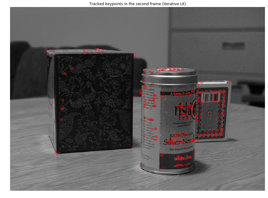
# Detect keypoints to track in the first frame
keypoints = corner_peaks(corner_harris(frames[0]),
                         exclude_border=5,
                         threshold_rel=0.01)

# Track keypoints using iterative Lucas-Kanade method
trajs = track_features(frames, keypoints,
                       error_thresh=1.5,
                       optflow_fn=iterative_lucas_kanade,
                       window_size=5)
ani = animated_scatter(frames,trajs)
HTML(ani.to_html5_video())

运行到最后，相比于之前LK光流，迭代式光流法追踪并保留了更多的关键点。

2.2 Coarse-to-Fine Optical Flow

The iterative method still could not track larger motions. If we downscaled the images, larger displacements would become easier to track. On the otherhand, smaller motions would become more difficult to track as we lose details in the images. To address this problem, we can represent images in multi-scale, and compute flow vectors from coarse to fine scale.

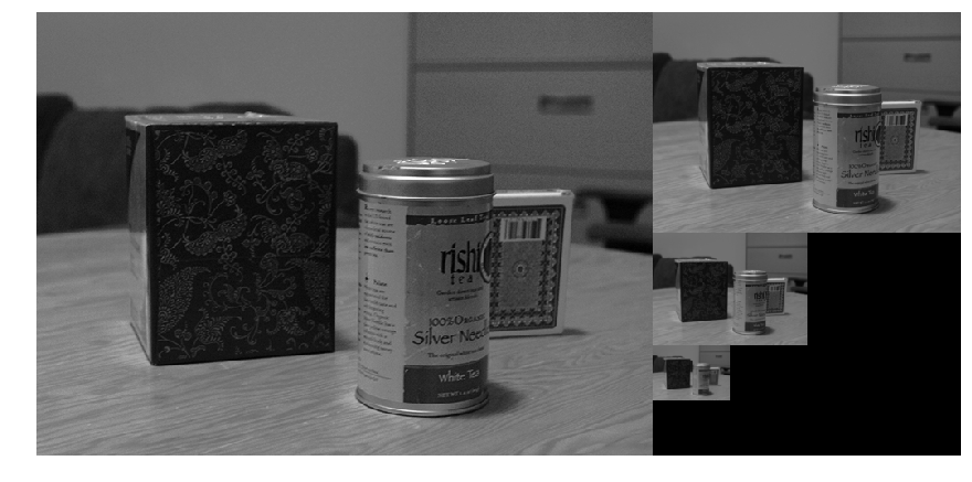
Run the following code cell to visualize image pyramid.

2.1的迭代金字塔方式依旧不能追踪更大的运动。

原因是因为，如果进行下采样得到的图像，大的运行是更容易追踪到了，但是另一方面，较小的运动却被忽略掉了，因为这部分信息被下采样给丢失了。

为了解决这个问题，这里使用多尺度来表征图像，并且从粗粒度到细粒度来计算光流。

#下面这段函数是使用skimage提供的函数来生成不同尺度的图像。

from skimage.transform import pyramid_gaussian

image = frames[0]

# pyramid_gaussian returns tuple of max_layer + 1 images in multiple scales
pyramid = tuple(pyramid_gaussian(image, max_layer=3, downscale=2))

rows, cols = image.shape
composite_image = np.zeros((rows, cols + cols // 2 + 1), dtype=np.double)
composite_image[:rows, :cols] = pyramid[0]

i_row = 0
for p in pyramid[1:]:
    n_rows, n_cols = p.shape
    composite_image[i_row:i_row + n_rows, cols:cols + n_cols] = p
    i_row += n_rows

# Display image pyramid
plt.figure(figsize=(15,12))
plt.imshow(composite_image)
plt.axis('off')
plt.show()

Following is the description of pyramidal Lucas-Kanade algorithm:

Let $p$ be a point on image $I$ and $s$ be the scale of pyramid representation.

• Build pyramid representations of $I$ and $J$: ${I^L}{L=0,…,L_m}$ and ${J^L}{L=0,…,L_m}$

• Initialize pyramidal guess

  $$ g^{L_m}= \begin{bmatrix}g_{x}^{L_m} & g_{y}^{L_m}\end{bmatrix}^T=\begin{bmatrix}0 & 0\end{bmatrix}^T $$

• for $L=L_m$ to $0$ with step of -1

  • Compute location of $p$ on $I^L$: $p^L=p/s^L$

  • Let $d^L$ be the optical flow vector at level $L$:

$$
d^L := IterativeLucasKanade(I^L, J^L, p^L, g^L)
$$
- Guess for next level $L-1$: $g^{L-1}=s(g^L+d^L)$

• Return $d=g^0+d^0$

Implement pyramid_lucas_kanade.

上面的是金字塔法Lukas-Kanade光流的算法描述

算法公式有了，原理还是没看懂，可能要追溯到论文去理解了。

from motion import pyramid_lucas_kanade

# Lucas-Kanade method for optical flow
flow_vectors = pyramid_lucas_kanade(frames[0], frames[1], keypoints)

# Plot flow vectors
plt.figure(figsize=(15,12))
plt.imshow(frames[0])
plt.axis('off')
plt.title('Optical flow vectors (pyramid LK)')

for y, x, vy, vx in np.hstack((keypoints, flow_vectors)):
    plt.arrow(x, y, vx, vy, head_width=3, head_length=3, color='b')

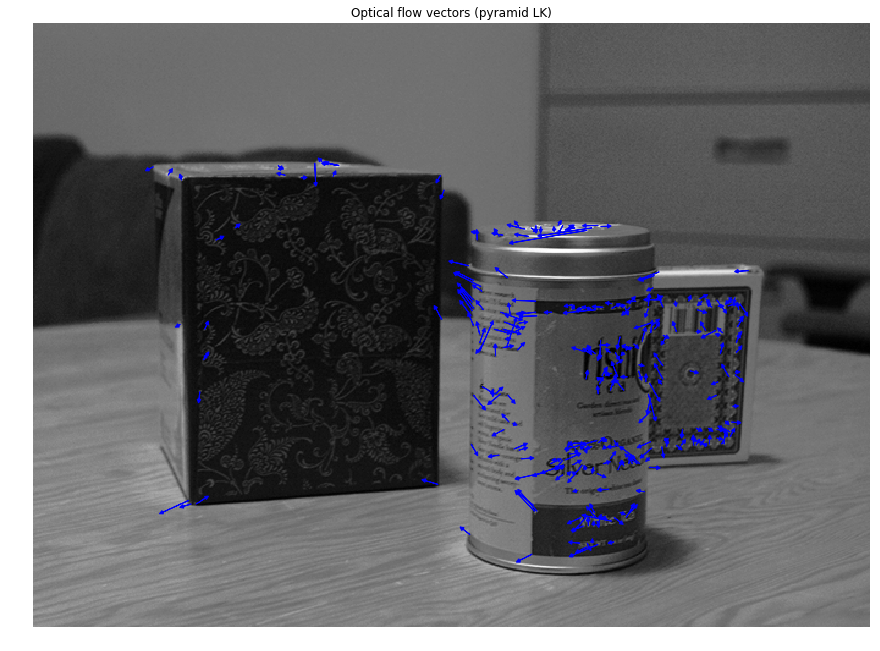
上图可知，金字塔方式LK光流既能检测到大运行，也能检测到小运动。但是幅度也太大了点。

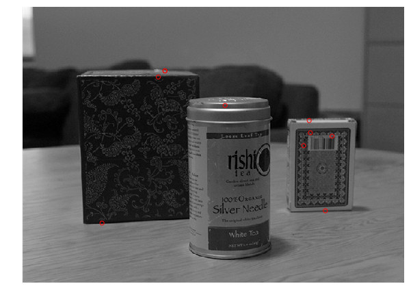
# Plot tracked kepoints
new_keypoints = keypoints + flow_vectors
plt.figure(figsize=(15,12))
plt.imshow(frames[1])
plt.scatter(new_keypoints[:,1], new_keypoints[:,0],
            facecolors='none', edgecolors='r')
plt.axis('off')
plt.title('Tracked keypoints in the second frame (pyramid LK)')

plt.show()

from utils import animated_scatter
from motion import track_features
keypoints = corner_peaks(corner_harris(frames[0]),
                         exclude_border=5,
                         threshold_rel=0.01)

trajs = track_features(frames, keypoints,
                       error_thresh=1.5,
                       optflow_fn=pyramid_lucas_kanade,
                       window_size=5)
ani = animated_scatter(frames,trajs)
HTML(ani.to_html5_video())

总体比较下来，金字塔法光流耗时最多。

效果不行啊，貌似第二帧关键点都追丢了，怀疑是计算得到的光流幅度太大引起的。

仔细检查了一遍算法实现，代码上应该木有问题，原理上出错了吗？？。

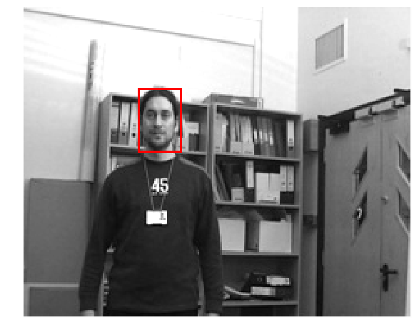
3. Object Tracking

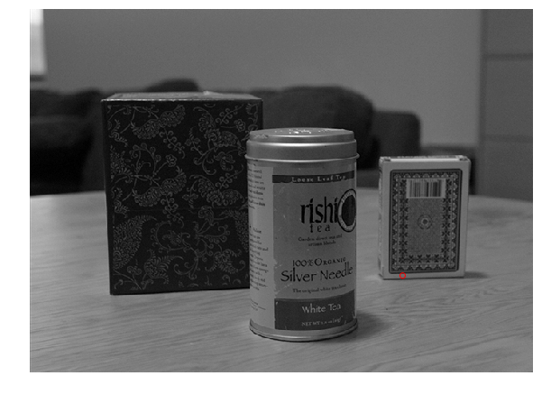
Let us build a simple object tracker using the Lucas-Kanade method we have implemented in previous sections. In order to test the object tracker, we provide you a short face-tracking sequence. Each frame in the sequence is annotated with the ground-truth location (as bounding box) of face.

An object tracker is given an object bounding box in the first frame, and it has to track the object by predicting bounding boxes in subsequent frames.

目标追踪

在第一帧中提供了目标的外包围框，要在接下来的帧序列中预测目标运行。

from utils import animated_bbox, load_bboxes

# Load frames and ground truth bounding boxes
frames = load_frames('Man/img')
gt_bboxes = load_bboxes('Man/groundtruth_rect.txt')

ani = animated_bbox(frames, gt_bboxes)
HTML(ani.to_html5_video())

In order to track the object, we first find keypoints to track inside the bounding box. Then, we track those points in each of the following frames and output a tight bounding box around the tracked points. In order to prevent all the keypoints being lost, we detect new keypoints within the bounding box every 20 frames.

1. 找到包围盒中的关键点。
2. 在接下来的帧中追踪这些关键点，并用包围盒框住这些关键点。
3. 为了防止关键点的消失，每二十帧进行一次关键点的检测。

# Find features to track within the bounding box
x, y, w, h = gt_bboxes[0]
roi = frames[0][y:y+h, x:x+w]
keypoints = corner_peaks(corner_harris(roi),
                         exclude_border=3,
                         threshold_rel=0.001)

# Shift keypoints by bbox offset
keypoints[:,1] += x
keypoints[:,0] += y

# Plot kepoints
plt.figure(figsize=(15,12))
plt.imshow(frames[0])
plt.scatter(keypoints[:,1], keypoints[:,0],
            facecolors='none', edgecolors='r')
plt.axis('off')
plt.show()

from motion import compute_error

# Initailze keypoints abd bounding box
kp_I = keypoints
x, y, w, h = gt_bboxes[0]
bboxes = [(x, y, w, h)]

for i in range(len(frames)-1):
    I = frames[i] # current frame
    J = frames[i+1] # next frame
    
    # estimate keypoints in frame J
    # 这里使用迭代式LK光流和金字塔LK光流进行测试
    flow_vectors = iterative_lucas_kanade(I, J, kp_I) #pyramid_lucas_kanade
    kp_J = kp_I + flow_vectors
    
    # Leave out lost points
    new_keypoints = []
    for yi, xi, yj, xj in np.hstack((kp_I, kp_J)):
        if yj > J.shape[0]-2 or yj < 1 or xj > J.shape[1]-2 or xj < 1:
            print('out of bound')
            continue
        else:
            patch_I = I[int(yi)-1:int(yi)+2, int(xi)-1:int(xi)+2]
            patch_J = J[int(yj)-1:int(yj)+2, int(xj)-1:int(xj)+2]
            error = compute_error(patch_I, patch_J)
            if error > 3.0:
                continue
            else:
                new_keypoints.append([yj, xj])
    
    # Update keypoints
    kp_I = np.array(new_keypoints)
    
    # Find bounding box around the keypoints
    if len(kp_I) > 0:
        x = int(kp_I[:,1].min())
        y = int(kp_I[:,0].min())
        w = int(kp_I[:,1].max()) - x
        h = int(kp_I[:,0].max()) - y
    else:
        (x, y, w, h) = (0, 0, 0, 0)
    bboxes.append((x,y,w,h))

    # Refresh keypoints every 20 frames
    if (i+1) % 20 == 0 and (w * h > 0):
        roi = J[y:y+h, x:x+w]
        new_keypoints = corner_peaks(corner_harris(roi),
                                 exclude_border=5,
                                 threshold_rel=0.01)
        new_keypoints[:,1] += x
        new_keypoints[:,0] += y
        kp_I = np.vstack((kp_I, new_keypoints))

ani = animated_bbox(frames, bboxes)
HTML(ani.to_html5_video())

金字塔光流法
到最后竟然包围盒消失了，两个原因吧

• 一个是特征点的检测算法对于光照敏感，
• 一个是光流追踪没有完善。
  其实，上一步金字塔光流法其实还没有解决问题哩。

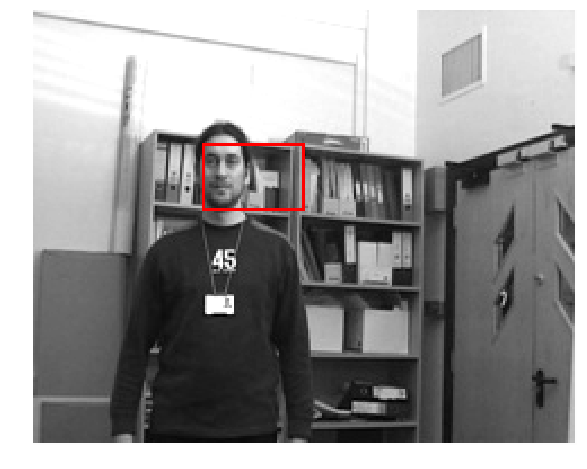
迭代光流法
IOU分数能达到0.32，但是明显的错误在于，在过程中更新关键点时，将复杂背景下的一些脸部之外的关键点包括了进来，导致了最后的追踪不仅包含了最开始的目标，还包括了复杂背景的一些关键点。

3.1 Evaluating Object Tracker: intersection over union (IoU)

Intersection over union is a common metric for evaluating performance of an object tracker. Implement IoU in motion.py to evaluate our object tracker. With default parameters, you will get IoU score of ~0.32.

根据真值，评估自己的追踪效果。
计算方法看图：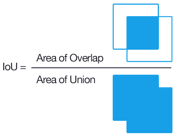

博客推荐

Intersection over Union (IoU) for object detection

from motion import IoU

average_iou = 0.0
for gt_bbox, bbox in zip(gt_bboxes, bboxes):
    average_iou += IoU(gt_bbox, bbox)
    
average_iou /= len(gt_bboxes)
print(average_iou)

0.32643400622199703

Extra Credit: Optimizing Object Tracker

Optimize object tracker in the code cell below. You may modify the code and define new parameters. We will grant extra credit for IoU score > 0.45.

这里要求改进，提高准确率。

我的思路就是,从上一视频的问题入手，错误的一个明显原因就是引入了复杂背景的一些关键点，所以一个解决方案就是避免引入这些关键点。

方案一：

1. 每隔20帧重新获取关键点
2. 对新的关键点进行筛选，保留与初始关键点最相似的点。其实就是根据找特征点的匹配。

这就需要对关键点进行描述了。当然，其实也可以对Harris检测角点这一方法换成别的关键点检测算法来做。

当然，由于金字塔光流法没能完成，我使用迭代式光流法做的实验。

from motion import compute_error

from skimage.feature import (match_descriptors, corner_peaks, corner_harris,
                             plot_matches, BRIEF)
from skimage.feature import match_template

### Define your parameters here
### Describe the paramters in comments
error_thresh = 3.0
n_frames = 20


#####################################################
# You may modify the code below to use the params you
# define above.
#####################################################

# Find features to track within the bounding box
x, y, w, h = gt_bboxes[0]
roi = frames[0][y:y+h, x:x+w]
keypoints = corner_peaks(corner_harris(roi),
                         exclude_border=3,
                         threshold_rel=0.001)

# Shift keypoints by bbox offset
keypoints[:,1] += x
keypoints[:,0] += y

# 改进标记,获取第一幅图的关键点描述子
extractor = BRIEF()
extractor.extract(frames[0], keypoints)
descriptorsOrigin = extractor.descriptors
# print(descriptorsOrigin.shape)

targetTemplete = roi

# Initailze keypoints and bounding box
kp_I = keypoints
x, y, w, h = gt_bboxes[0]
bboxes = [(x, y, w, h)]

# Start tracking
for i in range(len(frames)-1):
    I = frames[i] # Current frame
    J = frames[i+1] # Next frame
    flow_vectors = iterative_lucas_kanade(I, J, kp_I) # Compute flow vectors # 换成迭代法
    kp_J = kp_I + flow_vectors # Estimate keypoints in frame J
    
    new_keypoints = []
    for yi, xi, yj, xj in np.hstack((kp_I, kp_J)):
        # keypoint falls outside the image
        if yj > J.shape[0]-2 or yj < 1 or xj > J.shape[1]-2 or xj < 1:
            print('out of bound')
            continue
        else:
            # Compute error to find lost points
            patch_I = I[int(yi)-1:int(yi)+2, int(xi)-1:int(xi)+2]
            patch_J = J[int(yj)-1:int(yj)+2, int(xj)-1:int(xj)+2]
            error = compute_error(patch_I, patch_J)
            if error > error_thresh:
                continue
            else:
                new_keypoints.append([yj, xj])
    
    # Update keypoints
    kp_I = np.array(new_keypoints)
    
    # Find bounding box around the keypoints
    if len(kp_I) > 0:
        x = int(kp_I[:,1].min())
        y = int(kp_I[:,0].min())
        w = int(kp_I[:,1].max()) - x
        h = int(kp_I[:,0].max()) - y
    else:
        (x, y, w, h) = (0, 0, 0, 0)
  
    bboxes.append((x,y,w,h))

    # Detect new keypoints every n_frames
    if (i+1) % n_frames == 0 and (w * h > 0):
        roi = J[y:y+h, x:x+w]
        new_keypoints = corner_peaks(corner_harris(roi),
                                 exclude_border=5,
                                 threshold_rel=0.01)
        
        new_keypoints[:,1] += x
        new_keypoints[:,0] += y   
        
        # 新区域内的关键点数目
#         print(new_keypoints.shape)
        
        # 提取新区域内的关键点描述子
        extractor.extract(J, new_keypoints)
        descriptorsUpadte = extractor.descriptors
#         print(descriptorsUpadte.shape)
        
        # 匹配新区域关键点与初始关键点
        matches = match_descriptors(descriptorsOrigin, descriptorsUpadte, cross_check=True)
#         print(matches.shape)
        
#         print(matches)
#         print(matches[:,1])
#         print(new_keypoints)
#         print(new_keypoints[matches[:,1]])
        # 保留匹配到的关键点
        remainKeyPoints = new_keypoints[matches[:,1]]
        
                             
        kp_I = np.vstack((kp_I, remainKeyPoints))

/home/ubuntu/anaconda3/lib/python3.6/site-packages/skimage/feature/match.py:49: FutureWarning: Conversion of the second argument of issubdtype from `bool` to `np.generic` is deprecated. In future, it will be treated as `np.bool_ == np.dtype(bool).type`.
  if np.issubdtype(descriptors1.dtype, np.bool):

ani = animated_bbox(frames, bboxes)
HTML(ani.to_html5_video())

from motion import IoU

average_iou = 0.0
for gt_bbox, bbox in zip(gt_bboxes, bboxes):
    average_iou += IoU(gt_bbox, bbox)
    
average_iou /= len(gt_bboxes)
print(average_iou)

0.3901405329460035

方案一，将原来的0.32的准确率提高到了0.39，

但是同样有一个明显错误的地方就是，进行关键点匹配的时候，复杂的背景依旧提供了与初始关键点相似的点，使得这种方案并不是很完善。

代码档案

官方Repo作业材料

个人Repo作业存档

cs131学完咯，开始cs231n和Kaggle打比赛咯