CS131,Homewrok6,Recognition-Classification

Homework 6

This notebook includes both coding and written questions. Please hand in this notebook file with all the outputs as a pdf on gradescope for “HW6 pdf”. Upload the three files of code (compression.py, k_nearest_neighbor.py and features.py) on gradescope for “HW6 code”.

This assignment covers:

• image compression using SVD
• kNN methods for image recognition.
• PCA and LDA to improve kNN

这份任务包括了：

1. 使用SVD进行图像压缩
2. 使用kNN方法进行图像识别
3. 使用PCA和LDA提升kNN性能

# Setup
from time import time
from collections import defaultdict

import numpy as np
import matplotlib.pyplot as plt
from matplotlib import rc
from skimage import io

%matplotlib inline
plt.rcParams['figure.figsize'] = (15.0, 12.0) # set default size of plots
plt.rcParams['image.interpolation'] = 'nearest'
plt.rcParams['image.cmap'] = 'gray'

# for auto-reloading external modules
%load_ext autoreload
%autoreload 2

The autoreload extension is already loaded. To reload it, use:
  %reload_ext autoreload

Part 1 - Image Compression (15 points)

Image compression is used to reduce the cost of storage and transmission of images (or videos).
One lossy compression method is to apply Singular Value Decomposition (SVD) to an image, and only keep the top n singular values.

此处虽然称之为图像压缩，实际上就是数据处理里的降维的步骤。

有关SVD（奇异值分解），可以看这篇博客，博客都是我随便找的，看懂原理即可。

机器学习中的数学(5)-强大的矩阵奇异值分解(SVD)及其应用

image = io.imread('pitbull.jpg', as_grey=True)
plt.imshow(image)
plt.axis('off')
plt.show()

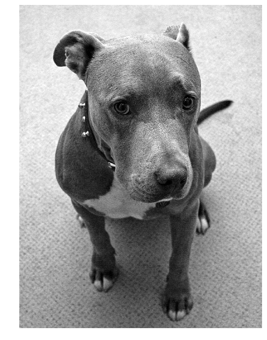
Let’s implement image compression using SVD.
We first compute the SVD of the image, and as seen in class we keep the n largest singular values and singular vectors to reconstruct the image.

Implement function compress_image in compression.py.

在compress_image函数中实现奇异值分解，并保留前N个较大的奇异值和对应的特征向量。

题目中的压缩率在我理解就是压缩后有效数据与压缩之前图像数据的比值。

from compression import compress_image

compressed_image, compressed_size = compress_image(image, 100)
compression_ratio = compressed_size / image.size
print('Original image shape:', image.shape)
print('Compressed size: %d' % compressed_size)
print('Compression ratio: %.3f' % compression_ratio)

assert compressed_size == 298500

Original image shape: (1704, 1280)
Compressed size: 298500
Compression ratio: 0.137

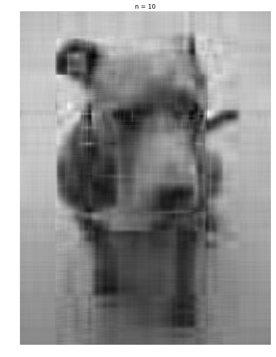
# Number of singular values to keep
n_values = [10, 50, 100]

for n in n_values:
    # Compress the image using `n` singular values
    compressed_image, compressed_size = compress_image(image, n)
    
    compression_ratio = compressed_size / image.size

    print("Data size (original): %d" % (image.size))
    print("Data size (compressed): %d" % compressed_size)
    print("Compression ratio: %f" % (compression_ratio))



    plt.imshow(compressed_image, cmap='gray')
    title = "n = %s" % n
    plt.title(title)
    plt.axis('off')
    plt.show()

Data size (original): 2181120
Data size (compressed): 29850
Compression ratio: 0.013686

Data size (original): 2181120
Data size (compressed): 149250
Compression ratio: 0.068428

Data size (original): 2181120
Data size (compressed): 298500
Compression ratio: 0.136856

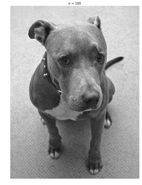
实现了用SVD实现了图像的压缩，同时可以发现：n=100时，压缩率0.13时，图像质量就已经很接近原图了。

这样看来，SVD的确用来做降维是很合适的。毕竟能够大大提高运行速度。

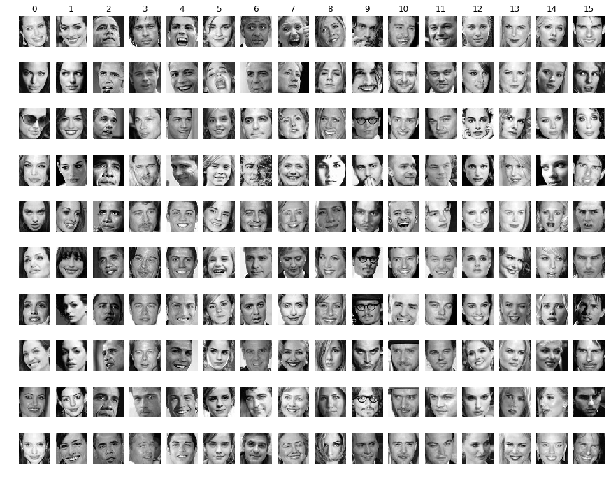
Face Dataset

We will use a dataset of faces of celebrities. Download the dataset using the following command:

sh get_dataset.sh

The face dataset for CS131 assignment.
The directory containing the dataset has the following structure:

faces/
    train/
        angelina jolie/
        anne hathaway/
        ...
    test/
        angelina jolie/
        anne hathaway/
        ...

Each class has 50 training images and 10 testing images.

命令行执行sh get_dataset.sh就可以下载了。

# 加载数据集
from utils import load_dataset

X_train, y_train, classes_train = load_dataset('faces', train=True, as_grey=True)
X_test, y_test, classes_test = load_dataset('faces', train=False, as_grey=True)

assert classes_train == classes_test
classes = classes_train

print('Class names:', classes)
print('Training data shape:', X_train.shape)
print('Training labels shape: ', y_train.shape)
print('Test data shape:', X_test.shape)
print('Test labels shape: ', y_test.shape)

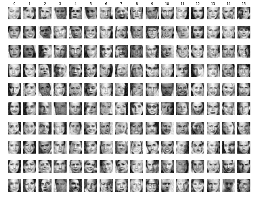
Class names: ['angelina jolie', 'anne hathaway', 'barack obama', 'brad pitt', 'cristiano ronaldo', 'emma watson', 'george clooney', 'hillary clinton', 'jennifer aniston', 'johnny depp', 'justin timberlake', 'leonardo dicaprio', 'natalie portman', 'nicole kidman', 'scarlett johansson', 'tom cruise']
Training data shape: (800, 64, 64)
Training labels shape:  (800,)
Test data shape: (160, 64, 64)
Test labels shape:  (160,)

# 可视化数据集中的一些样本
# 从每一类中显示一些样本
num_classes = len(classes)
samples_per_class = 10
for y, cls in enumerate(classes):
    idxs = np.flatnonzero(y_train == y)
    idxs = np.random.choice(idxs, samples_per_class, replace=False)
    for i, idx in enumerate(idxs):
        plt_idx = i * num_classes + y + 1
        plt.subplot(samples_per_class, num_classes, plt_idx)
        plt.imshow(X_train[idx])
        plt.axis('off')
        if i == 0:
            plt.title(y)
plt.show()

# 将图像数据展开为行，即每个样本为一行
# 这样每个样本我们就有了4096个维度的特征
X_train = np.reshape(X_train, (X_train.shape[0], -1))
X_test = np.reshape(X_test, (X_test.shape[0], -1))
print("Training data shape:", X_train.shape)
print("Test data shape:", X_test.shape)

Training data shape: (800, 4096)
Test data shape: (160, 4096)

---

Part 2 - k-Nearest Neighbor (30 points)

We’re now going to try to classify the test images using the k-nearest neighbors algorithm on the raw features of the images (i.e. the pixel values themselves). We will see later how we can use kNN on better features.

Here are the steps that we will follow:

1. We compute the L2 distances between every element of X_test and every element of X_train in compute_distances.
2. We split the dataset into 5 folds for cross-validation in split_folds.
3. For each fold, and for different values of k, we predict the labels and measure accuracy.
4. Using the best k found through cross-validation, we measure accuracy on the test set.

博客推荐

机器学习（一）——K-近邻（KNN）算法

kNN（k最近邻算法）的步骤如下：

1. 计算测试数据X_test中每个样本与训练数据X_train中每个样本之间的距离，距离计算方式为L2距离。
2. 将数据集分割为5Folder（5折）
3. 对每个子集和每个不同的参数k，预测结果并计算准确率
4. 通过交叉验证找到最佳的参数k，并在测试集上评估准确率

from k_nearest_neighbor import compute_distances

# Step 1: compute the distances between all features from X_train and from X_test
# 第一步：计算训练集和测试集上所有特征的距离（L2），调用cdist函数即可
dists = compute_distances(X_test, X_train)
assert dists.shape == (160, 800)
print("dists shape:", dists.shape)

dists shape: (160, 800)

预测结果分两步：

1. 找到预测点的最近的k个点
2. 判断k个点中频率最高的train_label

from k_nearest_neighbor import predict_labels

# We use k = 1 (which corresponds to only taking the nearest neighbor to decide)
y_test_pred = predict_labels(dists, y_train, k=1)

# Compute and print the fraction of correctly predicted examples
num_test = y_test.shape[0]
num_correct = np.sum(y_test_pred == y_test)
accuracy = float(num_correct) / num_test
print('Got %d / %d correct => accuracy: %f' % (num_correct, num_test, accuracy))

Got 38 / 160 correct => accuracy: 0.237500

Cross-Validation

We don’t know the best value for our parameter k.
There is no theory on how to choose an optimal k, and the way to choose it is through cross-validation.

We cannot compute any metric on the test set to choose the best k, because we want our final test accuracy to reflect a real use case. This real use case would be a setting where we have new examples come and we classify them on the go. There is no way to check the accuracy beforehand on that set of test examples to determine k.

Cross-validation will make use split the data into different fold (5 here).
For each fold, if we have a total of 5 folds we will have:

• 80% of the data as training data
• 20% of the data as validation data

We will compute the accuracy on the validation accuracy for each fold, and use the mean of these 5 accuracies to determine the best parameter k.

from k_nearest_neighbor import split_folds

# Step 2: split the data into 5 folds to perform cross-validation.
# 步骤二：分割数据为5折，执行交叉验证
num_folds = 5

X_trains, y_trains, X_vals, y_vals = split_folds(X_train, y_train, num_folds)

assert X_trains.shape == (5, 640, 4096)
assert y_trains.shape == (5, 640)
assert X_vals.shape == (5, 160, 4096)
assert y_vals.shape == (5, 160)

# Step 3: Measure the mean accuracy for each value of `k`
# 步骤三：计算每个参数k对应的平均准确率

# List of k to choose from
k_choices = list(range(5, 101, 5))

# Dictionnary mapping k values to accuracies
# For each k value, we will have `num_folds` accuracies to compute
# k_to_accuracies[1] will be for instance [0.22, 0.23, 0.19, 0.25, 0.20] for 5 folds
k_to_accuracies = {}

for k in k_choices:
    print("Running for k=%d" % k)
    accuracies = []
    for i in range(num_folds):
        # Make predictions
        fold_dists = compute_distances(X_vals[i], X_trains[i])
        y_pred = predict_labels(fold_dists, y_trains[i], k)

        # Compute and print the fraction of correctly predicted examples
        num_correct = np.sum(y_pred == y_vals[i])
        accuracy = float(num_correct) / len(y_vals[i])
        accuracies.append(accuracy)
        
    k_to_accuracies[k] = accuracies

Running for k=5
Running for k=10
Running for k=15
Running for k=20
Running for k=25
Running for k=30
Running for k=35
Running for k=40
Running for k=45
Running for k=50
Running for k=55
Running for k=60
Running for k=65
Running for k=70
Running for k=75
Running for k=80
Running for k=85
Running for k=90
Running for k=95
Running for k=100

# plot the raw observations
# 绘图进行观察
for k in k_choices:
    accuracies = k_to_accuracies[k]
    plt.scatter([k] * len(accuracies), accuracies)

# plot the trend line with error bars that correspond to standard deviation
# 
accuracies_mean = np.array([np.mean(v) for k,v in sorted(k_to_accuracies.items())])
accuracies_std = np.array([np.std(v) for k,v in sorted(k_to_accuracies.items())])
plt.errorbar(k_choices, accuracies_mean, yerr=accuracies_std)
plt.title('Cross-validation on k')
plt.xlabel('k')
plt.ylabel('Cross-validation accuracy')
plt.show()

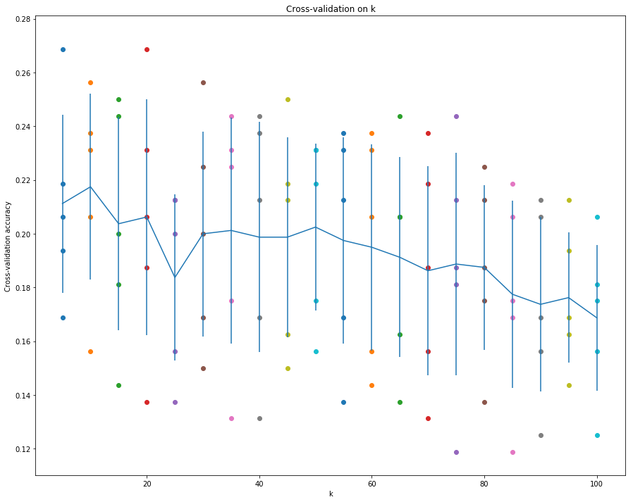
从这幅图看，前30之内有两个峰值就达到了最高的准确率和较好的标准差。

可以进一步细化step进行测试。

# Step 3: Measure the mean accuracy for each value of `k`
# 步骤三：计算每个参数k对应的平均准确率

# List of k to choose from
k_choices = list(range(1, 31, 1))

# Dictionnary mapping k values to accuracies
# For each k value, we will have `num_folds` accuracies to compute
# k_to_accuracies[1] will be for instance [0.22, 0.23, 0.19, 0.25, 0.20] for 5 folds
k_to_accuracies = {}

for k in k_choices:
    print("Running for k=%d" % k)
    accuracies = []
    for i in range(num_folds):
        # Make predictions
        fold_dists = compute_distances(X_vals[i], X_trains[i])
        y_pred = predict_labels(fold_dists, y_trains[i], k)

        # Compute and print the fraction of correctly predicted examples
        num_correct = np.sum(y_pred == y_vals[i])
        accuracy = float(num_correct) / len(y_vals[i])
        accuracies.append(accuracy)
        
    k_to_accuracies[k] = accuracies

Running for k=1
Running for k=2
Running for k=3
Running for k=4
Running for k=5
Running for k=6
Running for k=7
Running for k=8
Running for k=9
Running for k=10
Running for k=11
Running for k=12
Running for k=13
Running for k=14
Running for k=15
Running for k=16
Running for k=17
Running for k=18
Running for k=19
Running for k=20
Running for k=21
Running for k=22
Running for k=23
Running for k=24
Running for k=25
Running for k=26
Running for k=27
Running for k=28
Running for k=29
Running for k=30

# plot the raw observations
# 绘图进行观察
for k in k_choices:
    accuracies = k_to_accuracies[k]
    plt.scatter([k] * len(accuracies), accuracies)

# plot the trend line with error bars that correspond to standard deviation
# 
accuracies_mean = np.array([np.mean(v) for k,v in sorted(k_to_accuracies.items())])
accuracies_std = np.array([np.std(v) for k,v in sorted(k_to_accuracies.items())])
plt.errorbar(k_choices, accuracies_mean, yerr=accuracies_std)
plt.title('Cross-validation on k')
plt.xlabel('k')
plt.ylabel('Cross-validation accuracy')
plt.show()

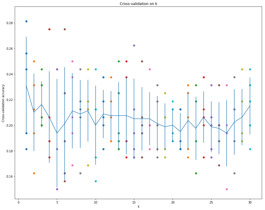
# Based on the cross-validation results above, choose the best value for k,   
# retrain the classifier using all the training data, and test it on the test
# data. You should be able to get above 26% accuracy on the test data.

best_k = None
# YOUR CODE HERE
# Choose the best k based on the cross validation above
best_k =2
# END YOUR CODE

y_test_pred = predict_labels(dists, y_train, k=best_k)

# Compute and display the accuracy
num_correct = np.sum(y_test_pred == y_test)
accuracy = float(num_correct) / num_test
print('For k = %d, got %d / %d correct => accuracy: %f' % (best_k, num_correct, num_test, accuracy))

For k = 2, got 42 / 160 correct => accuracy: 0.262500

既然k=2和k=17准确率相同，应该是选择k较小的，这样可以提高运行速率吧。

---

Part 3: PCA (30 points)

Principal Component Analysis (PCA) is a simple yet popular and useful linear transformation technique that is used in numerous applications, such as stock market predictions, the analysis of gene expression data, and many more. In this tutorial, we will see that PCA is not just a “black box”, and we are going to unravel its internals in 3 basic steps.

Introduction

The sheer size of data in the modern age is not only a challenge for computer hardware but also a main bottleneck for the performance of many machine learning algorithms. The main goal of a PCA analysis is to identify patterns in data; PCA aims to detect the correlation between variables. If a strong correlation between variables exists, the attempt to reduce the dimensionality only makes sense. In a nutshell, this is what PCA is all about: Finding the directions of maximum variance in high-dimensional data and project it onto a smaller dimensional subspace while retaining most of the information.

A Summary of the PCA Approach

• Standardize the data.
• Obtain the Eigenvectors and Eigenvalues from the covariance matrix or correlation matrix, or perform Singular Vector Decomposition.
• Sort eigenvalues in descending order and choose the $k$ eigenvectors that correspond to the $k$ largest eigenvalues where $k$ is the number of dimensions of the new feature subspace ($k \leq d$).
• Construct the projection matrix $\mathbf{W}$ from the selected $k$ eigenvectors.
• Transform the original dataset $\mathbf{X}$ via $\mathbf{W}$ to obtain a $k$-dimensional feature subspace Y.

博客推荐

浅谈对主成分分析（PCA）算法的理解

PCA方法（主成分分析）的总结

PCA的主旨就是：在高维数据中找到最大方差的方向，并将高维数据投射到低维的子空间，这样能够保留尽可能多的信息。

• 标准化数据
• 从协方差矩阵或互相关矩阵或者用SVD奇异值分解，来获得特征向量和特征值
• 将特征值降序排序，根据新特征空间的维度k，选择前k个最大的特征值和对应的特征向量（k <= d）
• 根据k个特征向量构建投影矩阵W
• 将数据集X通过W转换到k维的特征子空间

from features import PCA

pca = PCA()

3.1 - Eigendecomposition

The eigenvectors and eigenvalues of a covariance (or correlation) matrix represent the “core” of a PCA: The eigenvectors (principal components) determine the directions of the new feature space, and the eigenvalues determine their magnitude. In other words, the eigenvalues explain the variance of the data along the new feature axes.

Implement _eigen_decomp in pca.py.

特征向量和特征值代表了PCA的核心：

• 特征向量（主成分）决定了新的特征空间的方向
• 特征值决定了特征向量的幅度，换言之，特征值表示了数据在新特征方向的方差。方差越大，信息量越大。

博客推荐

协方差矩阵计算方法

# Perform eigenvalue decomposition on the covariance matrix of training data.
# 在训练数据的协方差矩阵上执行特征分解
t1 = time()
e_vecs, e_vals = pca._eigen_decomp(X_train - X_train.mean(axis=0))
t2 = time()

print(e_vals.shape)
print(e_vecs.shape)
print("耗时：", t2-t1)

(4096,)
(4096, 4096)
耗时： 32.20034837722778

直接解特征向量太慢了。

3.2 - Singular Value Decomposition

Doing an eigendecomposition of the covariance matrix is very expensive, especially when the number of features (D = 4096 here) gets very high.

To obtain the same eigenvalues and eigenvectors in a more efficient way, we can use Singular Value Decomposition (SVD). If we perform SVD on matrix $X$, we obtain $U$, $S$ and $V$ such that:
$$
X = U S V^T
$$

• the columns of $U$ are the eigenvectors of $X X^T$
• the columns of $V^T$ are the eigenvectors of $X^T X$
• the values of $S$ are the square roots of the eigenvalues of $X^T X$ (or $X X^T$)

Therefore, we can find out the top k eigenvectors of the covariance matrix $X^T X$ using SVD.

Implement _svd in pca.py.

这里讲到了直接利用协方差矩阵计算特征分解是非常耗时的事情，特别是维度很高的情况下。

其实更高效的方式是使用SVD（奇异值分解）。

具体的左奇异向量和右奇异向量与特征向量的对应关系在上面描述了，所以利用SVD就能得到特征向量和特征值

# Perform SVD on directly on the training data.
t1 = time()
u, s = pca._svd(X_train - X_train.mean(axis=0))
t2 = time()

print(s.shape)
print(u.shape)
print("耗时：", t2-t1)

(800,)
(4096, 4096)
耗时： 1.3446221351623535

# Test whether the square of singular values and eigenvalues are the same.
# We also observe that `e_vecs` and `u` are the same (only the sign of each column can differ).
# 这里测试直接分解协方差矩阵和使用SVD方法得到的是否相同
N = X_train.shape[0]
assert np.allclose((s ** 2) / (N - 1), e_vals[:len(s)])

for i in range(len(s) - 1):
    assert np.allclose(e_vecs[:, i], u[:, i]) or np.allclose(e_vecs[:, i], -u[:, i])
    # (the last eigenvector for i = len(s) - 1 is very noisy because the eigenvalue is almost 0,
    #  so imprecisions in the computation build up)

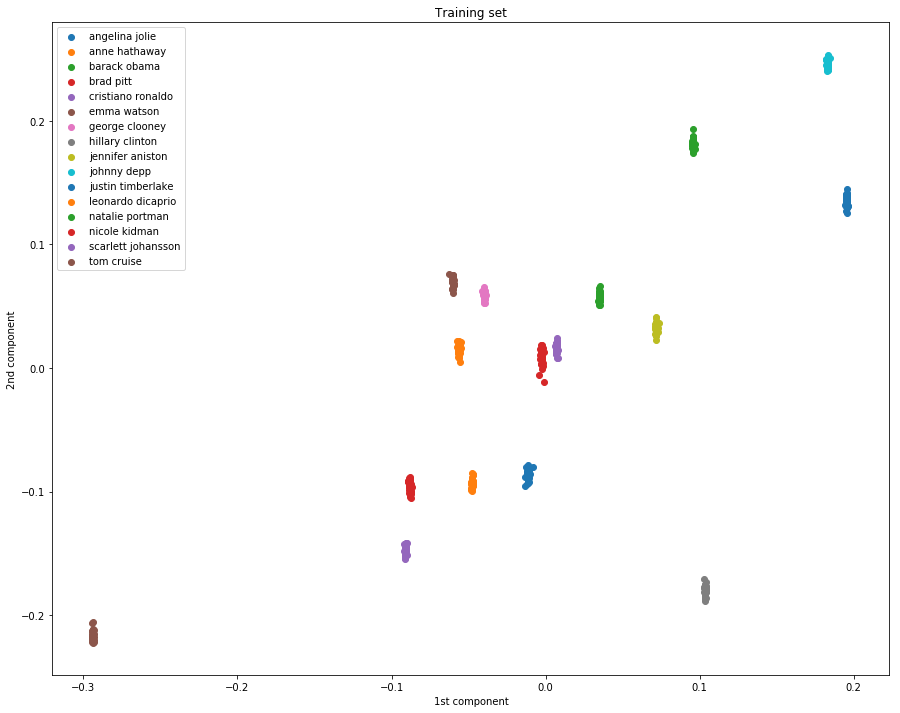
3.3 - Dimensionality Reduction

The top $k$ principal components explain most of the variance of the underlying data.

By projecting our initial data (the images) onto the subspace spanned by the top k principal components,
we can reduce the dimension of our inputs while keeping most of the information.

In the example below, we can see that using the first two components in PCA is not enough to allow us to see pattern in the data. All the classes seem placed at random in the 2D plane.

维度缩减

通过将前k个主成分投影在子空间，就可以达到缩减维度的目的，同时能够保留最大的信息。

需要在feature.py中实现 transform 函数，同时在fit函数中实现X的均值计算。

# Dimensionality reduction by projecting the data onto
# lower dimensional subspace spanned by k principal components

# To visualize, we will project in 2 dimensions
n_components = 2
pca.fit(X_train)
X_proj = pca.transform(X_train, n_components)

# Plot the top two principal components
for y in np.unique(y_train):
    plt.scatter(X_proj[y_train==y,0], X_proj[y_train==y,1], label=classes[y])
    
plt.xlabel('1st component')
plt.ylabel('2nd component')
plt.legend()
plt.show()

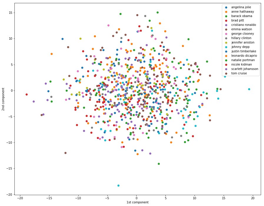
一脸懵逼，这里我们可以看到，仅仅用两个最大的主成分是无法看出数据的特征来的。

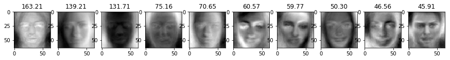
3.4 - Visualizing Eigenfaces

The columns of the PCA projection matrix pca.W_pca represent the eigenvectors of $X^T X$.

We can visualize the biggest singular values as well as the corresponding vectors to get a sense of what the PCA algorithm is extracting.

If we visualize the top 10 eigenfaces, we can see tht the algorithm focuses on the different shades of the faces. For instance, in face n°2 the light seems to come from the left.

for i in range(10):
    plt.subplot(1, 10, i+1)
    plt.imshow(pca.W_pca[:, i].reshape(64, 64))
    plt.title("%.2f" % s[i])
plt.show()

# Reconstruct data with principal components
# 利用主成分进行数据重构，重构实际上就是投影的逆向操作。
n_components = 100  # 测试不同的参数值查看对重构的影响
X_proj = pca.transform(X_train, n_components)
X_rec = pca.reconstruct(X_proj)

print(X_rec.shape)
print(classes)

# 查看重构后的脸部图像
samples_per_class = 10
for y, cls in enumerate(classes):
    idxs = np.flatnonzero(y_train == y)
    idxs = np.random.choice(idxs, samples_per_class, replace=False)
    for i, idx in enumerate(idxs):
        plt_idx = i * num_classes + y + 1
        plt.subplot(samples_per_class, num_classes, plt_idx)
        plt.imshow((X_rec[idx]).reshape((64, 64)))
        plt.axis('off')
        if i == 0:
            plt.title(y)
plt.show()

(800, 4096)
['angelina jolie', 'anne hathaway', 'barack obama', 'brad pitt', 'cristiano ronaldo', 'emma watson', 'george clooney', 'hillary clinton', 'jennifer aniston', 'johnny depp', 'justin timberlake', 'leonardo dicaprio', 'natalie portman', 'nicole kidman', 'scarlett johansson', 'tom cruise']

哈哈，100个主成分能够分清男女了，200个主成分大概能够分清是哪个人了。

Written Question 1 (5 points)

Question: Consider a dataset of $N$ face images, each with shape $(h, w)$. Then, we need $O(Nhw)$ of memory to store the data. Suppose we perform dimensionality reduction on the dataset with $p$ principal components, and use the components as bases to represent images. Calculate how much memory we need to store the images and the matrix used to get back to the original space.

Said in another way, how much memory does storing the compressed images and the uncompresser cost.

Answer: TODO

问题：压缩的图像占用的内存空间和解压器需要占用的内存空间

答：

1. 降维后的图像维度为 X_proj.shape = (N, n_components)，所以实际压缩的图像占用空间即为$O(Np)$

2. 为了实现压缩和复原的其他资源（姑且称之为解压器），需要保存的变量包括self.W_pca和self.mean，实际上内存大头就是样本的所有主成分表，所以解压器占用的内存空间为$O(pD)$ = $O(phw)$

3.5 - Reconstruction error and captured variance

We can plot the reconstruction error with respect to the dimension of the projected space.

The reconstruction gets better with more components.

We can see in the plot that the inflexion point is around dimension 200 or 300. This means that using this number of components is a good compromise between good reconstruction and low dimension.

# Plot reconstruction errors for different k
# 绘制出不同主成分数目对应的重构误差
N = X_train.shape[0]
d = X_train.shape[1]

ns = range(1, d, 20)
errors = []

for n in ns:
    X_proj = pca.transform(X_train, n)
    X_rec = pca.reconstruct(X_proj)

    # Compute reconstruction error
    error = np.mean((X_rec - X_train) ** 2)
    errors.append(error)

plt.plot(ns, errors)
plt.xlabel('Number of Components')
plt.ylabel('Reconstruction Error')
plt.show()

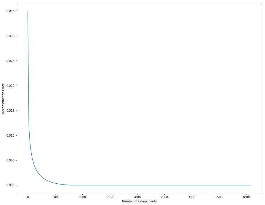
从上面这幅图可以获取到的有用信息就是：

1. 1000以内，误差随着主成分数目增加而减小
2. 大概在200-400间，出现了下降速率的拐角，此处可以来个权衡，因为主成分数目并不是越多越好，它影响了运行的效率。选择拐角处的值，既能保证误差率较低，还能兼顾计算时间。

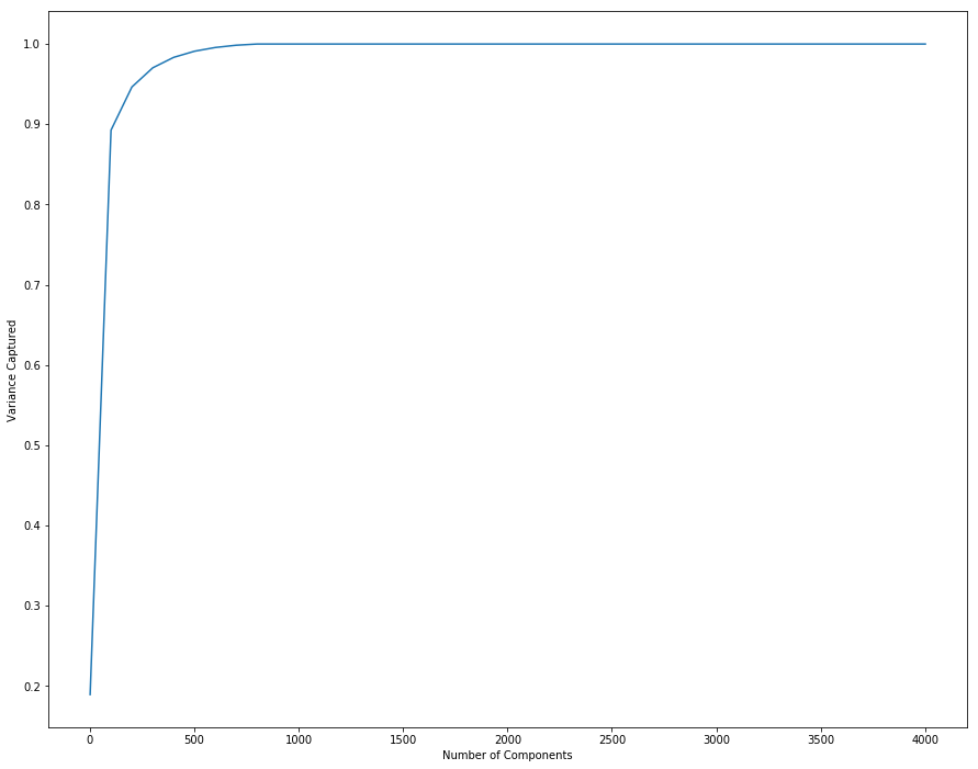
We can do the same process to see how much variance is captured by the projection.

Again, we see that the inflexion point is around 200 or 300 dimensions.

同样，方差的拐点也在200-400之间

# Plot captured variance
ns = range(1, d, 100)
var_cap = []

for n in ns:
    var_cap.append(np.sum(s[:n] ** 2)/np.sum(s ** 2))
    
plt.plot(ns, var_cap)
plt.xlabel('Number of Components')
plt.ylabel('Variance Captured')
plt.show()

3.6 - kNN with PCA

Performing kNN on raw features (the pixels of the image) does not yield very good results.
Computing the distance between images in the image space is not a very good metric for actual proximity of images.
For instance, an image of person A with a dark background will be close to an image of B with a dark background, although these people are not the same.

Using a technique like PCA can help discover the real interesting features and perform kNN on them could give better accuracy.

However, we observe here that PCA doesn’t really help to disentangle the features and obtain useful distance metrics between the different classes. We basically obtain the same performance as with raw features.

上面这段话讲的挺好，直接使用原始的特征（即图像的像素）并不能表现的很好，因为在计算图像之间的距离时，两个不同物体具有相同的黑色背景时，背景明显在计算上减小了两者之间的距离，虽然我们要判断的是前景的类别。

使用PCA能够得到有趣的特征，能够使kNN能够达到更高的准确率。

但是，在这里，PCA并不能在不同类别里区分开特征，获取到有用的距离。这里看起来和使用像素是一样的效果。

num_test = X_test.shape[0]

# We computed the best k and n for you
best_k = 20
best_n = 100


# PCA
pca = PCA()
pca.fit(X_train)
X_proj = pca.transform(X_train, best_n)
X_test_proj = pca.transform(X_test, best_n)

# kNN
dists = compute_distances(X_test_proj, X_proj)
y_test_pred = predict_labels(dists, y_train, k=best_k)

# Compute and display the accuracy
num_correct = np.sum(y_test_pred == y_test)
accuracy = float(num_correct) / num_test
print('Got %d / %d correct => accuracy: %f' % (num_correct, num_test, accuracy))

Got 45 / 160 correct => accuracy: 0.281250

呵呵哒，我知道PCA有用，但就涨了这么点准确率，我怎么能信服。

---

Part 4 - Fisherface: Linear Discriminant Analysis (25 points)

LDA is a linear transformation method like PCA, but with a different goal.
The main difference is that LDA takes information from the labels of the examples to maximize the separation of the different classes in the transformed space.

Therefore, LDA is not totally unsupervised since it requires labels. PCA is fully unsupervised.

In summary:

• PCA perserves maximum variance in the projected space.
• LDA preserves discrimination between classes in the project space. We want to maximize scatter between classes and minimize scatter intra class.

博客推荐

机器学习中的数学(4)-线性判别分析（LDA）, 主成分分析(PCA)

如何理解LDA算法？能够简洁明了地说明一下LDA算法的中心思想吗？

LDA和PCA的区别

LDA的主旨就是从标签中获取信息，在转换的目标空间最大化不同种类之间的隔离。

盗了一张图作说明，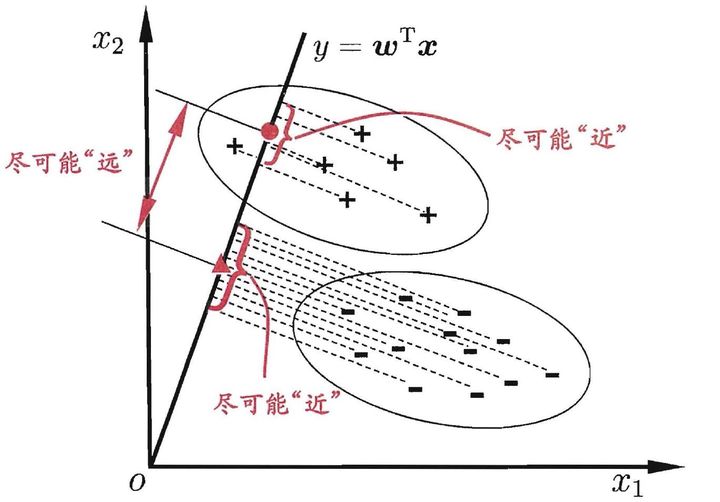

from features import LDA

lda = LDA()

4.1 - Dimensionality Reduction via PCA

To apply LDA, we need $D < N$. Since in our dataset, $N = 800$ and $D = 4096$, we first need to reduce the number of dimensions of the images using PCA.
More information at: http://www.scholarpedia.org/article/Fisherfaces

通过PCA实现维度的缩减

这里提到数据特征维度要比样本数少，所以需要进行一步特征的维度缩减，就直接拿PCA做降维好了。

N = X_train.shape[0]
c = num_classes

pca = PCA()
pca.fit(X_train)
X_train_pca = pca.transform(X_train, N-c)
X_test_pca = pca.transform(X_test, N-c)

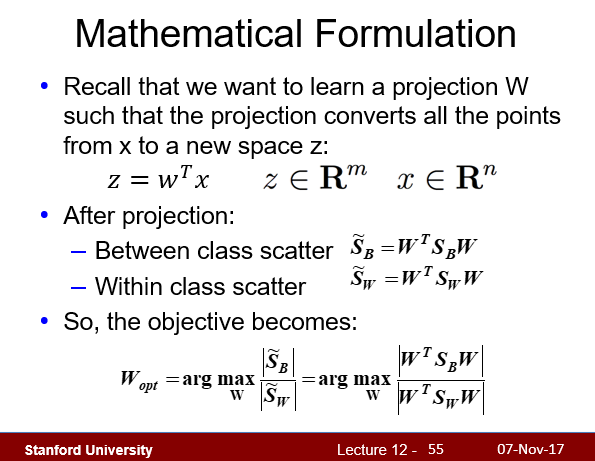
4.2 - Scatter matrices

We first need to compute the within-class scatter matrix:
$$
S_W = \sum_{i=1}^c S_i
$$
where $S_i = \sum_{x_k \in Y_i} (x_k - \mu_i)(x_k - \mu_i)^T$ is the scatter of class $i$.

We then need to compute the between-class scatter matrix:
$$
S_B = \sum_{i=1}^c N_i (\mu_i - \mu)(\mu_i - \mu)^T
$$
where $N_i$ is the number of examples in class $i$.

头疼的数学：散点图矩阵

上面的公式偏向结论的，具体的推导在Lecture13 的PPT 第42页开始。

# Compute within-class scatter matrix
# 计算类内散点图矩阵
S_W = lda._within_class_scatter(X_train_pca, y_train)
print(S_W.shape)

(784, 784)

# Compute between-class scatter matrix
# 计算类间散点图矩阵
S_B = lda._between_class_scatter(X_train_pca, y_train)
print(S_B.shape)

(784, 784)

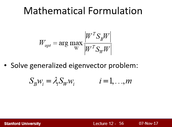
4.3 - Solving generalized Eigenvalue problem

Implement methods fit and transform of the LDA class.

哈哈，根据课堂PPT第55页，最终将优化问题泛化为了一个求特征值的问题。编程时直接使用线性代数库求解特征值即可。

lda.fit(X_train_pca, y_train)

# Dimensionality reduction by projecting the data onto
# lower dimensional subspace spanned by k principal components
# 通过K个主成分，将数据投射到低维的子空间上来实现维度缩减
# 这个实现方式其实跟PCA应该是一样的
n_components = 2
X_proj = lda.transform(X_train_pca, n_components)

X_test_proj = lda.transform(X_test_pca, n_components)

# Plot the top two principal components on the training set
for y in np.unique(y_train):
    plt.scatter(X_proj[y_train==y, 0], X_proj[y_train==y, 1], label=classes[y])
    
plt.xlabel('1st component')
plt.ylabel('2nd component')
plt.legend()
plt.title("Training set")
plt.show()

# Plot the top two principal components on the test set
for y in np.unique(y_test):
    plt.scatter(X_test_proj[y_test==y, 0], X_test_proj[y_test==y,1], label=classes[y])
    
plt.xlabel('1st component')
plt.ylabel('2nd component')
plt.legend()
plt.title("Test set")
plt.show()

第一幅图的效果好是因为已经fit过了，即进行过了训练。

第二幅图的效果不好，泛化能力明显不行。

实现维度缩减的最后一步，投射到子空间的方式和PCA是一样的，

那么PCA和LDA唯一的不同就是寻找主成分的理念不同了，

PCA强调的是在实现维度缩减的同时最大化保留的信息量

LDA强调的则是最小化类内的区别，最大化类间的区别

4.4 - kNN with LDA

Thanks to having the information from the labels, LDA gives a discriminant space where the classes are far apart from each other.
This should help kNN a lot, as the job should just be to find the obvious 10 clusters.

However, as we’ve seen in the previous plot (section 4.3), the training data gets clustered pretty well, but the test data isn’t as nicely clustered as the training data (overfitting?).

Perform cross validation following the code below (you can change the values of k_choices and n_choices to search). Using the best result from cross validation, obtain the test accuracy.

LDA具有最大化类间差距最小化类内差距的功效，所以在分类问题能够有很大帮助

num_folds = 5

X_trains, y_trains, X_vals, y_vals = split_folds(X_train, y_train, num_folds)

k_choices = [1, 5, 10, 20]
n_choices = [5, 10, 20, 50, 100, 200, 500]

# k_choices = [5,6,7,8,9,10,11,12,13,14,15,16,17,18,19,20,21,22]
# n_choices = [10,11,12,13,14,15,16,17,18,19,20,21,22,23,24,25]


pass


# n_k_to_accuracies[(n, k)] should be a list of length num_folds giving the different
# accuracy values that we found when using that value of n and k.
n_k_to_accuracies = defaultdict(list)

for i in range(num_folds):
    # Fit PCA
    pca = PCA()
    pca.fit(X_trains[i])
    
    N = len(X_trains[i])
    X_train_pca = pca.transform(X_trains[i], N-c)
    X_val_pca = pca.transform(X_vals[i], N-c)
    
    # Fit LDA
    lda = LDA()
    lda.fit(X_train_pca, y_trains[i])
    
    for n in n_choices:
        X_train_proj = lda.transform(X_train_pca, n)
        X_val_proj = lda.transform(X_val_pca, n)

        dists = compute_distances(X_val_proj, X_train_proj)
            
        for k in k_choices:
            y_pred = predict_labels(dists, y_trains[i], k=k)

            # Compute and print the fraction of correctly predicted examples
            num_correct = np.sum(y_pred == y_vals[i])
            accuracy = float(num_correct) / len(y_vals[i])
            n_k_to_accuracies[(n, k)].append(accuracy)


for n in n_choices:
    print()
    for k in k_choices:
        accuracies = n_k_to_accuracies[(n, k)]
        print("For n=%d, k=%d: average accuracy is %f" % (n, k, np.mean(accuracies)))

For n=5, k=1: average accuracy is 0.150000
For n=5, k=5: average accuracy is 0.142500
For n=5, k=10: average accuracy is 0.146250
For n=5, k=20: average accuracy is 0.140000

For n=10, k=1: average accuracy is 0.153750
For n=10, k=5: average accuracy is 0.152500
For n=10, k=10: average accuracy is 0.153750
For n=10, k=20: average accuracy is 0.151250

For n=20, k=1: average accuracy is 0.172500
For n=20, k=5: average accuracy is 0.180000
For n=20, k=10: average accuracy is 0.176250
For n=20, k=20: average accuracy is 0.191250

For n=50, k=1: average accuracy is 0.161250
For n=50, k=5: average accuracy is 0.181250
For n=50, k=10: average accuracy is 0.183750
For n=50, k=20: average accuracy is 0.172500

For n=100, k=1: average accuracy is 0.160000
For n=100, k=5: average accuracy is 0.172500
For n=100, k=10: average accuracy is 0.165000
For n=100, k=20: average accuracy is 0.150000

For n=200, k=1: average accuracy is 0.166250
For n=200, k=5: average accuracy is 0.180000
For n=200, k=10: average accuracy is 0.183750
For n=200, k=20: average accuracy is 0.168750

For n=500, k=1: average accuracy is 0.167500
For n=500, k=5: average accuracy is 0.162500
For n=500, k=10: average accuracy is 0.180000
For n=500, k=20: average accuracy is 0.181250

# Based on the cross-validation results above, choose the best value for k,   
# retrain the classifier using all the training data, and test it on the test
# data. You should be able to get above 40% accuracy on the test data.

best_k = None
best_n = None
# YOUR CODE HERE
# Choose the best k based on the cross validation above
best_k =20
best_n = 500
# END YOUR CODE

N = len(X_train)

# Fit PCA
pca = PCA()
pca.fit(X_train)
X_train_pca = pca.transform(X_train, N-c)
X_test_pca = pca.transform(X_test, N-c)

# Fit LDA
lda = LDA()
lda.fit(X_train_pca, y_train)

# Project using LDA
X_train_proj = lda.transform(X_train_pca, best_n)
X_test_proj = lda.transform(X_test_pca, best_n)

dists = compute_distances(X_test_proj, X_train_proj)
y_test_pred = predict_labels(dists, y_train, k=best_k)

# Compute and display the accuracy
num_correct = np.sum(y_test_pred == y_test)
accuracy = float(num_correct) / num_test
print("For k=%d and n=%d" % (best_k, best_n))
print('Got %d / %d correct => accuracy: %f' % (num_correct, num_test, accuracy))

For k=20 and n=500
Got 36 / 160 correct => accuracy: 0.225000

一脸懵逼。说好的准确率的提升没有上去。感觉过程中没有问题啊
我估计这次训练得到的LDA泛化能力不行，就跟上面那个测试一样。

代码档案

官方Repo作业材料

个人Repo作业存档