CS131, Homewrok1, Filters-Instagram

Homework 1

This notebook includes both coding and written questions. Please hand in this notebook file with all the outputs and your answers to the written questions.

这份作业覆盖的主题有线性滤波器，卷积和互相关性。

# Setup
import numpy as np
import matplotlib.pyplot as plt
from time import time
from skimage import io

from __future__ import print_function

%matplotlib inline
plt.rcParams['figure.figsize'] = (10.0, 8.0) # set default size of plots
plt.rcParams['image.interpolation'] = 'nearest'
plt.rcParams['image.cmap'] = 'gray'

# for auto-reloading extenrnal modules
%load_ext autoreload
%autoreload 2

Part 1: Convolutions

1.1 Commutative Property (10 points)

Recall that the convolution of an image $f:\mathbb{R}^2\rightarrow \mathbb{R}$ and a kernel $h:\mathbb{R}^2\rightarrow\mathbb{R}$ is defined as follows:

$$
(f*h)[m,n]=\sum_{i=-\infty}^\infty\sum_{j=-\infty}^\infty f[i,j]\cdot h[m-i,n-j]
$$

Or equivalently,

\begin{align} (f*h)[m,n] &= \sum_{i=-\infty}^\infty\sum_{j=-\infty}^\infty h[i,j]\cdot f[m-i,n-j]\\ &= (h*f)[m,n] \end{align}

Show that this is true (i.e. prove that the convolution operator is commutative: $fh = hf$).

Your Answer: Write your solution in this markdown cell. Please write your equations in LaTex equations.

题目就是证明卷积交换律。

证明：
将式中积分变量 $i$ 和 $j$ 置换为 $m-x$ 和 $n-y$，则

\begin{align} (f*h)[m,n]&=\sum_{i=-\infty}^\infty\sum_{j=-\infty}^\infty f[i,j]\cdot h[m-i,n-j] \\ &=\sum_{x=+\infty}^{-\infty}\sum_{y=+\infty}^{-\infty} f[m-x,n-y]\cdot h[x,y] \\ &=\sum_{x=+\infty}^{-\infty}\sum_{y=+\infty}^{-\infty} h[x,y]\cdot f[m-x,n-y] \\ &=\sum_{x=-\infty}^{\infty}\sum_{y=-\infty}^{\infty} h[x,y]\cdot f[m-x,n-y] \\ &=(h*f)[m,n] \end{align}

证毕。

1.2 Linear and Shift Invariance (10 points)

Let $f$ be a function $\mathbb{R}^2\rightarrow\mathbb{R}$. Consider a system $f\xrightarrow{s}g$, where $g=(f*h)$ with some kernel $h:\mathbb{R}^2\rightarrow\mathbb{R}$. Show that $S$ defined by any kernel $h$ is a Linear Shift Invariant (LSI) system. In other words, for any $h$, show that $S$ satisfies both of the following:

• $S[a\cdot{f_1}+b\cdot{f_2}]= a\cdot{S[f_1]}+b\cdot{S[f_2]}$
• If $f[m,n]\xrightarrow{s}g[m,n]$ then $f[m-m_0,n-n_0]\xrightarrow{s}g[m-m_0,n-n_0]$

Your Answer: Write your solution in this markdown cell. Please write your equations in LaTex equations.

第一题证明：

\begin{align} S[a\cdot{f_1}+b\cdot{f_2}] &= [a\cdot{f_1}+b\cdot{f_2}]*h[m,n]\\ &=\sum_{i=-\infty}^\infty\sum_{j=-\infty}^\infty (a\cdot f_1[i,j]+b \cdot f_2[i,j])\cdot h[m-i,n-j] \\ &=\sum_{i=-\infty}^\infty\sum_{j=-\infty}^\infty (a \cdot f_1[i,j] \cdot h[m-i,n-j] + b \cdot f_2[i,j] \cdot h[m-i,n-j]) \\ &= a \cdot \sum_{i=-\infty}^\infty\sum_{j=-\infty}^\infty f_1[i,j] \cdot h[m-i,n-j] + b \cdot \sum_{i=-\infty}^\infty\sum_{j=-\infty}^\infty f_2[i,j] \cdot h[m-i,n-j] \\ &=a \cdot (f_1*h) + b \cdot (f_2*h) \\ &= a \cdot S[f_1] + b\cdot S[f_2] \end{align}

证毕.

第二题没证,不知道怎么证明线性移不别.

1.3 Implementation (30 points)

In this section, you will implement two versions of convolution:

• conv_nested
• conv_fast

First, run the code cell below to load the image to work with.

# Open image as grayscale
img = io.imread('dog.jpg', as_grey=True)

# Show image
plt.imshow(img)
plt.axis('off')
plt.title("Isn't he cute?")
plt.show()

Now, implement the function conv_nested in filters.py. This is a naive implementation of convolution which uses 4 nested for-loops. It takes an image $f$ and a kernel $h$ as inputs and outputs the convolved image $(f*h)$ that has the same shape as the input image. This implementation should take a few seconds to run.

• Hint: It may be easier to implement $(h*f)$

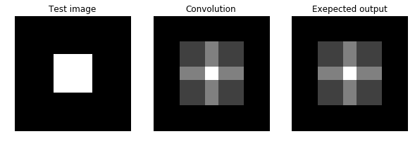
We’ll first test your conv_nested function on a simple input.

思路：使用四层嵌套循环来实现对图像的卷积操作。
两种方案：

• 按照卷积函数的公式定义来进行计算。

  $$
  (f*h)[m,n]=\sum_{i=-\infty}^\infty\sum_{j=-\infty}^\infty f[i,j]\cdot h[m-i,n-j]
  $$

• 按照卷积计算的可视化过程进行计算，即翻转内核，移动内核，累加迭代的过程。

conv_nested的实现在filters.py中。

from filters import conv_nested

# Simple convolution kernel.
kernel = np.array(
[
    [1,0,1],
    [0,0,0],
    [1,0,1]
])

# Create a test image: a white square in the middle
test_img = np.zeros((9, 9))
test_img[3:6, 3:6] = 1

# Run your conv_nested function on the test image
test_output = conv_nested(test_img, kernel)

# Build the expected output
expected_output = np.zeros((9, 9))
expected_output[2:7, 2:7] = 1
expected_output[4, 2:7] = 2
expected_output[2:7, 4] = 2
expected_output[4, 4] = 4

# Plot the test image
plt.subplot(1,3,1)
plt.imshow(test_img)
plt.title('Test image')
plt.axis('off')

# Plot your convolved image
plt.subplot(1,3,2)
plt.imshow(test_output)
plt.title('Convolution')
plt.axis('off')

# Plot the exepected output
plt.subplot(1,3,3)
plt.imshow(expected_output)
plt.title('Exepected output')
plt.axis('off')
plt.show()

# Test if the output matches expected output
assert np.max(test_output - expected_output) < 1e-10, "Your solution is not correct."

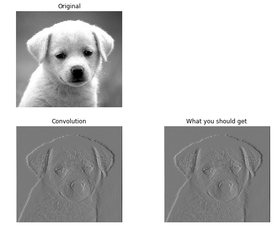
Now let’s test your conv_nested function on a real image.

简单的卷积测试，这是一个X方向上的边缘检测算子。

from filters import conv_nested

# Simple convolution kernel.
# Feel free to change the kernel and to see different outputs.
kernel = np.array(
[
    [1,0,-1],
    [2,0,-2],
    [1,0,-1]
])

out = conv_nested(img, kernel)

# Plot original image
plt.subplot(2,2,1)
plt.imshow(img)
plt.title('Original')
plt.axis('off')

# Plot your convolved image
plt.subplot(2,2,3)
plt.imshow(out)
plt.title('Convolution')
plt.axis('off')

# Plot what you should get
solution_img = io.imread('convoluted_dog.jpg', as_grey=True)
plt.subplot(2,2,4)
plt.imshow(solution_img)
plt.title('What you should get')
plt.axis('off')


plt.show()

Let us implement a more efficient version of convolution using array operations in numpy. As shown in the lecture, a convolution can be considered as a sliding window that computes sum of the pixel values weighted by the flipped kernel. The faster version will i) zero-pad an image, ii) flip the kernel horizontally and vertically, and iii) compute weighted sum of the neighborhood at each pixel.

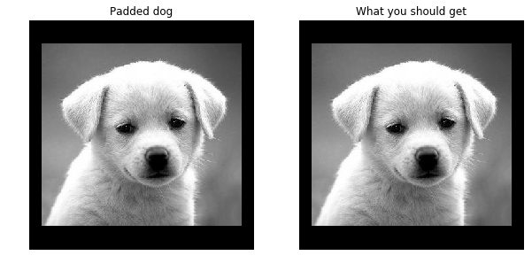
First, implement the function zero_pad in filters.py.

由于判断卷积核是否超出图像边界这一步导致计算很慢，这里有一种更快的方式：

1. 对图像边缘进行零填充
2. 翻转卷积核
3. 移动卷积核计算每个像素位置的卷积结果

零填充的操作就两步：

1. 根据填充边缘大小生成一个大背景
2. 将原图拷贝到背景中心

from filters import zero_pad

pad_width = 20 # width of the padding on the left and right
pad_height = 40 # height of the padding on the top and bottom

padded_img = zero_pad(img, pad_height, pad_width)

# Plot your padded dog
plt.subplot(1,2,1)
plt.imshow(padded_img)
plt.title('Padded dog')
plt.axis('off')

# Plot what you should get
solution_img = io.imread('padded_dog.jpg', as_grey=True)
plt.subplot(1,2,2)
plt.imshow(solution_img)
plt.title('What you should get')
plt.axis('off')

plt.show()

Next, complete the function conv_fast in filters.py using zero_pad. Run the code below to compare the outputs by the two implementations. conv_fast should run significantly faster than conv_nested.
Depending on your implementation and computer, conv_nested should take a few seconds and conv_fast should be around 5 times faster.

from filters import conv_fast

t0 = time()
out_fast = conv_fast(img, kernel)
t1 = time()
out_nested = conv_nested(img, kernel)
t2 = time()

# Compare the running time of the two implementations
print("conv_nested: took %f seconds." % (t2 - t1))
print("conv_fast: took %f seconds." % (t1 - t0))

# Plot conv_nested output
plt.subplot(1,2,1)
plt.imshow(out_nested)
plt.title('conv_nested')
plt.axis('off')

# Plot conv_fast output
plt.subplot(1,2,2)
plt.imshow(out_fast)
plt.title('conv_fast')
plt.axis('off')

# Make sure that the two outputs are the same
if not (np.max(out_fast - out_nested) < 1e-10):
    print("Different outputs! Check your implementation.")

conv_nested: took 5.063853 seconds.
conv_fast: took 1.080498 seconds.

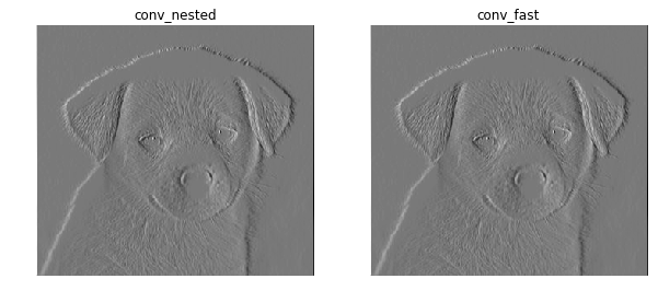
的确实现了约5倍大小的运行速度提升，需要指出的是，5倍的提升是（零填充+翻转卷积核计算）相对于（越界判断+卷积公式计算）来的。

经过测试，如果conv_nested是通过（翻转卷积核计算+越界判断）方式的话，本身运行时间大约在1.4s左右。

Extra Credit 1 (1% of final grade)

Devise a faster version of convolution and implement conv_faster in filters.py. You will earn extra credit only if the conv_faster runs faster (by a fair margin) than conv_fast and outputs the same result.

如何实现更快的卷积计算？ 我才想起来吴恩达在Machine Learning里特别强调了向量化带来的计算效率的提高。

参考了文章【算法+图像处理】2D卷积与快速卷积算法C语言实现，

偷看了一眼mikucy的作业，

向量化的思路就是：

1. 将卷积核进行向量化
2. 将迭代过程中的计算块（计算中心及其领域）进行向量化，由于运算的对象都是核，此处可以将向量化的计算块拼成矩阵
3. 两者进行内积计算，并reshape成原有图像大小

计算过程中的维度对齐：

• image: $(H_i,W_i)$
• kernel: $(H_k,W_k)$
• kernel_vectorized: $(H_k\cdot W_k,1)$
• patch_vectorized: $(1, H_k\cdot W_k)$
• image_vectorized2Matrix: $(H_i\cdot W_i, H_k\cdot W_k)$
• image_vectorized2Matrix * kernel_vectorized: $(H_i\cdot W_i,1)$
• reshaped: $(H_i,W_i)$

from filters import conv_faster

t0 = time()
out_fast = conv_fast(img, kernel)
t1 = time()
out_faster = conv_faster(img, kernel)
t2 = time()

# Compare the running time of the two implementations
print("conv_fast: took %f seconds." % (t1 - t0))
print("conv_faster: took %f seconds." % (t2 - t1))

# Plot conv_nested output
plt.subplot(1,2,1)
plt.imshow(out_fast)
plt.title('conv_fast')
plt.axis('off')

# Plot conv_fast output
plt.subplot(1,2,2)
plt.imshow(out_faster)
plt.title('conv_faster')
plt.axis('off')

# Make sure that the two outputs are the same
if not (np.max(out_fast - out_faster) < 1e-10):
    print("Different outputs! Check your implementation.")

conv_fast: took 1.084435 seconds.
conv_faster: took 0.310908 seconds.

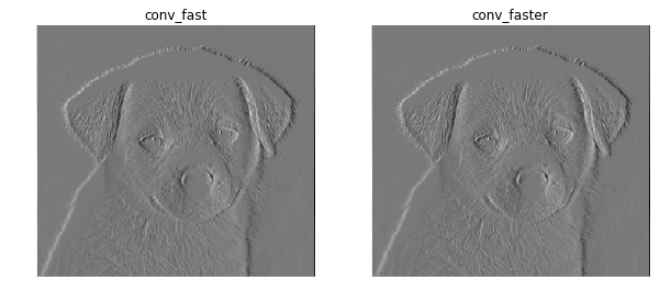
经过测试，向量化之后的卷积操作的确又快了5倍左右。不错不错。

---

Part 2: Cross-correlation

Cross-correlation of two 2D signals $f$ and $g$ is defined as follows:

$$
(f\star{g})[m,n]=\sum_{i=-\infty}^\infty\sum_{j=-\infty}^\infty f[i,j]\cdot g[i-m,j-n]
$$

2.1 Template Matching with Cross-correlation (12 points)

使用互相关性实现模板匹配

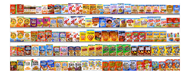
Suppose that you are a clerk at a grocery store. One of your responsibilites is to check the shelves periodically and stock them up whenever there are sold-out items. You got tired of this laborious task and decided to build a computer vision system that keeps track of the items on the shelf.

Luckily, you have learned in CS131 that cross-correlation can be used for template matching: a template $g$ is multiplied with regions of a larger image $f$ to measure how similar each region is to the template.

The template of a product (template.jpg) and the image of shelf (shelf.jpg) is provided. We will use cross-correlation to find the product in the shelf.

Implement cross_correlation function in filters.py and run the code below.

- Hint: you may use the conv_fast function you implemented in the previous question.

note 可以使用之前的卷积函数来进行计算，但要注意卷积里面对卷积核进行翻转，而计算互相关时，匹配模板如同滤波一样，并不需要翻转匹配模板。

from filters import cross_correlation

# Load template and image in grayscale
img = io.imread('shelf.jpg')
img_grey = io.imread('shelf.jpg', as_grey=True)
temp = io.imread('template.jpg')
temp_grey = io.imread('template.jpg', as_grey=True)

# Perform cross-correlation between the image and the template
out = cross_correlation(img_grey, temp_grey)

# Find the location with maximum similarity
y,x = (np.unravel_index(out.argmax(), out.shape))

# Display product template
plt.figure(figsize=(25,20))
plt.subplot(3, 1, 1)
plt.imshow(temp)
plt.title('Template')
plt.axis('off')

# Display cross-correlation output
plt.subplot(3, 1, 2)
plt.imshow(out)
plt.title('Cross-correlation (white means more correlated)')
plt.axis('off')

# Display image
plt.subplot(3, 1, 3)
plt.imshow(img)
plt.title('Result (blue marker on the detected location)')
plt.axis('off')

# Draw marker at detected location
plt.plot(x, y, 'bx', ms=40, mew=10)
plt.show()

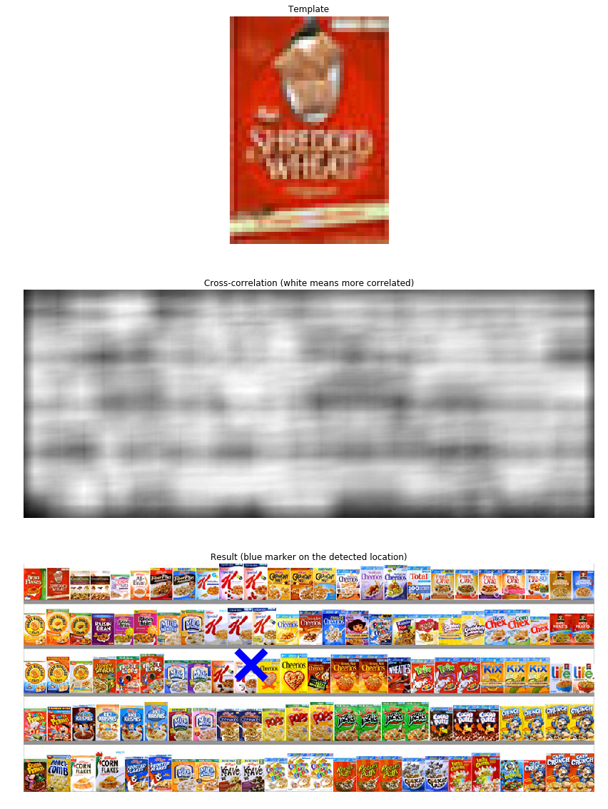
这里程序用了找匹配结果的最大值来判断匹配目标的所在。

Interpretation

How does the output of cross-correlation filter look like? Was it able to detect the product correctly? Explain what might be the problem with using raw template as a filter.

Your Answer: Write your solution in this markdown cell.

不是很清楚为啥不做任何处理匹配效果会很差。

• 一个可能是图像和模板的亮度不同导致了匹配的出错。
• 还有一个问题就是，一般的滤波核每个元素和加起来为一的，这个匹配图像作为内核去做计算的，肯定计算结果爆炸了呀，都是趋于255了？能量有种不协调的感觉

---

2.2 Zero-mean cross-correlation (6 points)

A solution to this problem is to subtract off the mean value of the template so that it has zero mean.

Implement zero_mean_cross_correlation function in filters.py and run the code below.

一种解决方案就是对匹配模板做零均值的操作。

from filters import zero_mean_cross_correlation

# Perform cross-correlation between the image and the template
out = zero_mean_cross_correlation(img_grey, temp_grey)

# Find the location with maximum similarity
y,x = (np.unravel_index(out.argmax(), out.shape))

# Display product template
plt.figure(figsize=(30,20))
plt.subplot(3, 1, 1)
plt.imshow(temp)
plt.title('Template')
plt.axis('off')

# Display cross-correlation output
plt.subplot(3, 1, 2)
plt.imshow(out)
plt.title('Cross-correlation (white means more correlated)')
plt.axis('off')

# Display image
plt.subplot(3, 1, 3)
plt.imshow(img)
plt.title('Result (blue marker on the detected location)')
plt.axis('off')

# Draw marker at detcted location
plt.plot(x, y, 'bx', ms=40, mew=10)
plt.show()

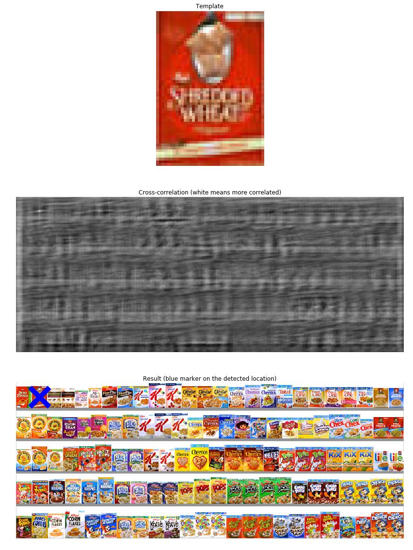
这样看来对匹配模板对零均值操作效果奇佳啊。

You can also determine whether the product is present with appropriate scaling and thresholding.

增加缩放和阈值来做判断。
阈值可以理解，不知道缩放的意义在于什么？

def check_product_on_shelf(shelf, product):
    out = zero_mean_cross_correlation(shelf, product)
    
    # Scale output by the size of the template
    out = out / float(product.shape[0]*product.shape[1])
    
    # Threshold output (this is arbitrary, you would need to tune the threshold for a real application)
    out = out > 0.025
    
    if np.sum(out) > 0:
        print('The product is on the shelf')
    else:
        print('The product is not on the shelf')

# Load image of the shelf without the product
img2 = io.imread('shelf_soldout.jpg')
img2_grey = io.imread('shelf_soldout.jpg', as_grey=True)

plt.imshow(img)
plt.axis('off')
plt.show()
check_product_on_shelf(img_grey, temp_grey)

plt.imshow(img2)
plt.axis('off')
plt.show()
check_product_on_shelf(img2_grey, temp_grey)

The product is on the shelf

The product is not on the shelf

---

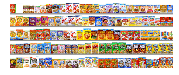
2.3 Normalized Cross-correlation (12 points)

One day the light near the shelf goes out and the product tracker starts to malfunction. The zero_mean_cross_correlation is not robust to change in lighting condition. The code below demonstrates this.

from filters import normalized_cross_correlation

# Load image
img = io.imread('shelf_dark.jpg')
img_grey = io.imread('shelf_dark.jpg', as_grey=True)


# Perform cross-correlation between the image and the template
out = zero_mean_cross_correlation(img_grey, temp_grey)

# Find the location with maximum similarity
y,x = (np.unravel_index(out.argmax(), out.shape))

# Display image
plt.imshow(img)
plt.title('Result (red marker on the detected location)')
plt.axis('off')

# Draw marker at detcted location
plt.plot(x, y, 'rx', ms=25, mew=5)
plt.show()

A solution is to normalize the pixels of the image and template at every step before comparing them. This is called normalized cross-correlation.

The mathematical definition for normalized cross-correlation of $f$ and template $g$ is:

$$
(f\star{g})[m,n]=\sum_{i,j} \frac{f[i,j]-\overline{f_{m,n}}}{\sigma_{f_{m,n}}} \cdot \frac{g[i-m,j-n]-\overline{g}}{\sigma_g}
$$

where:

• $f_{m,n}$ is the patch image at position $(m,n)$
• $\overline{f_{m,n}}$ is the mean of the patch image $f_{m,n}$
• $\sigma_{f_{m,n}}$ is the standard deviation of the patch image $f_{m,n}$
• $\overline{g}$ is the mean of the template $g$
• $\sigma_g$ is the standard deviation of the template $g$

Implement normalized_cross_correlation function in filters.py and run the code below.

直接对整幅待匹配的图做归一化操作，实验下来效果不行。

分析下来也是，正确的图像区域，如果是做整幅图的归一化的话，明显受到了其他区域诸如亮度颜色等的影响，干扰了匹配。

按照题目的意思是应该对每个待匹配块做归一化操作，然后比较匹配程度。

from filters import normalized_cross_correlation

# Perform normalized cross-correlation between the image and the template
out = normalized_cross_correlation(img_grey, temp_grey)

# Find the location with maximum similarity
y,x = (np.unravel_index(out.argmax(), out.shape))

# Display image
plt.imshow(img)
plt.title('Result (red marker on the detected location)')
plt.axis('off')

# Draw marker at detcted location
plt.plot(x, y, 'rx', ms=25, mew=5)
plt.show()

遍历的方式太慢，太耗时间了。我怀疑这种做法了。

Part 3: Separable Filters

3.1 Theory (10 points)

Consider a $M_1\times{N_1}$ image $I$ and a $M_2\times{N_2}$ filter $F$. A filter $F$ is separable if it can be written as a product of two 1D filters: $F=F_1F_2$.

For example,

$$
F=
\begin{bmatrix}
1 & -1 \\
1 & -1
\end{bmatrix}
$$

can be written as a matrix product of

$$
F_1=
\begin{bmatrix}
1 \\
1
\end{bmatrix},
F_2=
\begin{bmatrix}
1 & -1
\end{bmatrix}
$$

Therefore $F$ is a separable filter.

Prove that for any separable filter $F=F_1F_2$, $I*F=(I*F_1)*F_2$

Your Answer: Write your solution in this markdown cell. Please write your equations in LaTex equations.

证明

\begin{align} (I*F)[M_2,N_2] &= \sum_{i=-\infty}^\infty \sum_{j=-\infty}^\infty I[i,j]\cdot F[M_2-i,N_2-j] \tag{1}\\ &= \sum_{i=-\infty}^\infty\sum_{j=-\infty}^\infty I[i,j]\cdot F_1[M_2-i]\cdot F_2[N_2-j]\\ &= \sum_{j=-\infty}^\infty F_2[N_2-j] \cdot (\sum_{i=-\infty}^\infty I[i,j]\cdot F_1[M_2-i]) \tag{2}\\ &= \sum_{j=-\infty}^\infty F_2[N_2-j]\cdot(I(j)*F_1)\\ &= F_2 * (I * F_1) \\ &= (I * F_1) * F_2 \end{align}

证毕

3.2 Complexity comparison (10 points)

(i) How many multiplications do you need to do a direct 2D convolution (i.e. $I*F$?)

(ii) How many multiplications do you need to do 1D convolutions on rows and columns (i.e. $(I*F_1)*F_2$)

(iii) Use Big-O notation to argue which one is more efficient in general: direct 2D convolution or two successive 1D convolutions?

Your Answer: Write your solution in this markdown cell. Please write your equations in LaTex equations.

复杂度比较
根据上面的推导，可以看到式(1) 和 式(2)的区别：

1. $I*F$乘法操作的次数为 $M_1 \cdot N_1$
2. $(I*F_1)*F_2$乘法操作的次数为 $M_1+ N_1$
3. 我不会Big-O啊，明显分解的效率高哇。

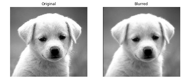
Now, we will empirically compare the running time of a separable 2D convolution and its equivalent two 1D convolutions. Gaussian kernel, widely used for blurring images, is one example of a separable filter. Run the code below to see its effect.

# Load image
img = io.imread('dog.jpg', as_grey=True)

# 5x5 Gaussian blur
kernel = np.array(
[
    [1,4,6,4,1],
    [4,16,24,16,4],
    [6,24,36,24,6],
    [4,16,24,16,4],
    [1,4,6,4,1]
])

t0 = time()
out = conv_nested(img, kernel)
t1 = time()
t_normal = t1 - t0

# Plot original image
plt.subplot(1,2,1)
plt.imshow(img)
plt.title('Original')
plt.axis('off')

# Plot convolved image
plt.subplot(1,2,2)
plt.imshow(out)
plt.title('Blurred')
plt.axis('off')

plt.show()

In the below code cell, define the two 1D arrays (k1 and k2) whose product is equal to the Gaussian kernel.

# The kernel can be written as outer product of two 1D filters
k1 = None  # shape (5, 1)
k2 = None  # shape (1, 5)

### YOUR CODE HERE
k1 = np.array([[1],[4],[6],[4],[1]])
k2 = np.array([[1,4,6,4,1]])

### END YOUR CODE

# Check if kernel is product of k1 and k2
if not  np.all(k1 * k2 == kernel):
    print('k1 * k2 is not equal to kernel')
    
assert k1.shape == (5, 1), "k1 should have shape (5, 1)"
assert k2.shape == (1, 5), "k2 should have shape (1, 5)"

We now apply the two versions of convolution to the same image, and compare their running time. Note that the outputs of the two convolutions must be the same.

# Perform two convolutions using k1 and k2
t0 = time()
out_separable = conv_nested(img, k1)
out_separable = conv_nested(out_separable, k2)
t1 = time()
t_separable = t1 - t0

# Plot normal convolution image
plt.subplot(1,2,1)
plt.imshow(out)
plt.title('Normal convolution')
plt.axis('off')

# Plot separable convolution image
plt.subplot(1,2,2)
plt.imshow(out_separable)
plt.title('Separable convolution')
plt.axis('off')

plt.show()

print("Normal convolution: took %f seconds." % (t_normal))
print("Separable convolution: took %f seconds." % (t_separable))

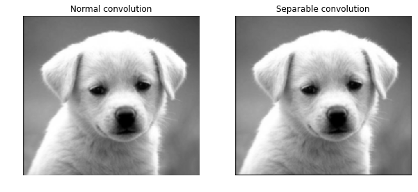
Normal convolution: took 13.643008 seconds.
Separable convolution: took 5.948668 seconds.

# Check if the two outputs are equal
assert np.max(out_separable - out) < 1e-10

# 肉眼看不出来哪有区别，不知为啥断言错误。

代码档案

官方Repo作业材料

个人Repo作业存档